---
title: "Transformer Foundations"
description: "Build the intuition and technical foundations to understand the Transformer, modern LLMs and VLMs, and their evolving architectures."
---
> Documentation Index
> Fetch the complete documentation index at: https://latentlit.com/llms.txt
> Use this file to discover all available pages before exploring further.
# Transformer Foundations
import FocusCanvas from '../../../components/FocusCanvas.astro';
import FoundationDiagram from '../../../components/architectures/FoundationDiagram.astro';
import EncoderDecoderFlow from '../../../components/architectures/EncoderDecoderFlow.astro';
import AttentionFlow from '../../../components/architectures/AttentionFlow.astro';
import SourceFigure from '../../../components/architectures/SourceFigure.astro';
This page builds a foundational understanding of the Transformer: a starting
point for studying modern large language models (LLMs), vision language models
(VLMs), and the architectures that come next.
Start with a simple idea: turn one sequence into another, as [Figure 1](#figure-1)
illustrates. A sentence becomes a
translation, a document becomes a summary, and a question becomes an answer.
This **sequence to sequence** formulation brings many language tasks under one
framework.[^t5] It can also reach beyond text: an image can become a sequence
describing the objects it contains and where they are.[^pix2seq] The original
Transformer was designed for translation, but the broader idea is a useful
starting point: represent an input and learn to produce the desired output.[^transformer]
Doing this well requires context. “Bank” means something different beside
“river” than beside “account.” A Transformer builds numerical representations
of its input, then refines them through repeated layers. Each position draws
on relevant information from the context it is allowed to see.[^transformer]
The design also suits large scale training. Unlike recurrent models, which
process a sequence through dependent steps, a Transformer can process many
positions together using matrix operations that run efficiently on GPUs.[^transformer]
Researchers can grow the model through more layers and wider representations;
studies have found predictable improvements in text prediction as model size,
data, and compute increase within tested ranges.[^scaling-laws] This is not
unlimited: comparing all pairs of positions is costly for long contexts, and ordinary
text generation still proceeds one token at a time.[^transformer]
We follow the original architecture, connect it to Harvard NLP's readable
implementation, and then look at modern LLMs and VLMs. Each component is
introduced when it becomes useful.
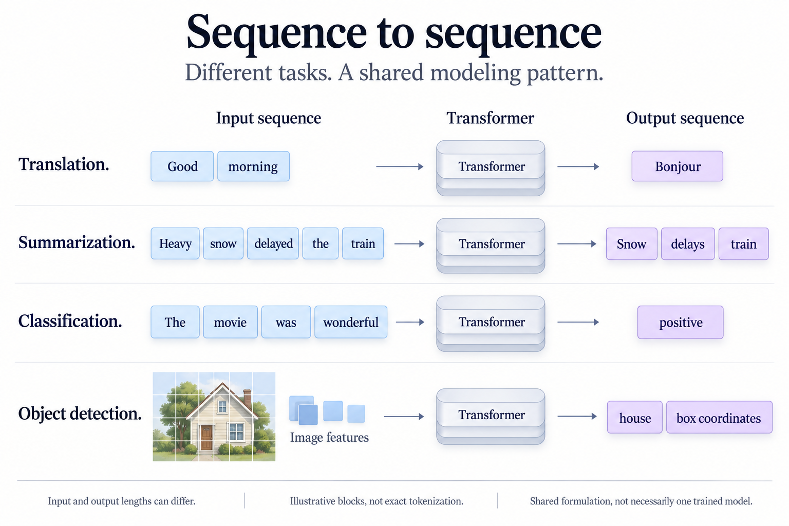
**Figure 1.** Different tasks, a shared sequence formulation. AI generated illustration informed by Transformer, T5, and Pix2Seq.[^transformer][^t5][^pix2seq]
**Image description:** Four left to right examples show input sequences passing through separate Transformer blocks to produce a translation, a summary, a classification label, or object labels and box coordinates from image features.
| Reading path | What to understand |
| --- | --- |
| [Architecture and data flow](#architecture-and-data-flow) | Two streams, encoder memory, decoder states, vocabulary scores |
| [Attention and masking](#attention-and-masking) | Q, K, V, scaling, softmax, visibility, head shapes, KV sharing |
| [Components and full model](#components-and-full-model) | Residuals, normalization, FFN, embeddings, position, independent layers |
| [Training and inference](#training-and-inference) | Shifted labels, loss, optimization, SFT, decoding, caching |
| [From Transformer to modern LLMs](#from-transformer-to-modern-llms) | Which contracts persist and which design choices change |
## Architecture and data flow
### Read the original architecture
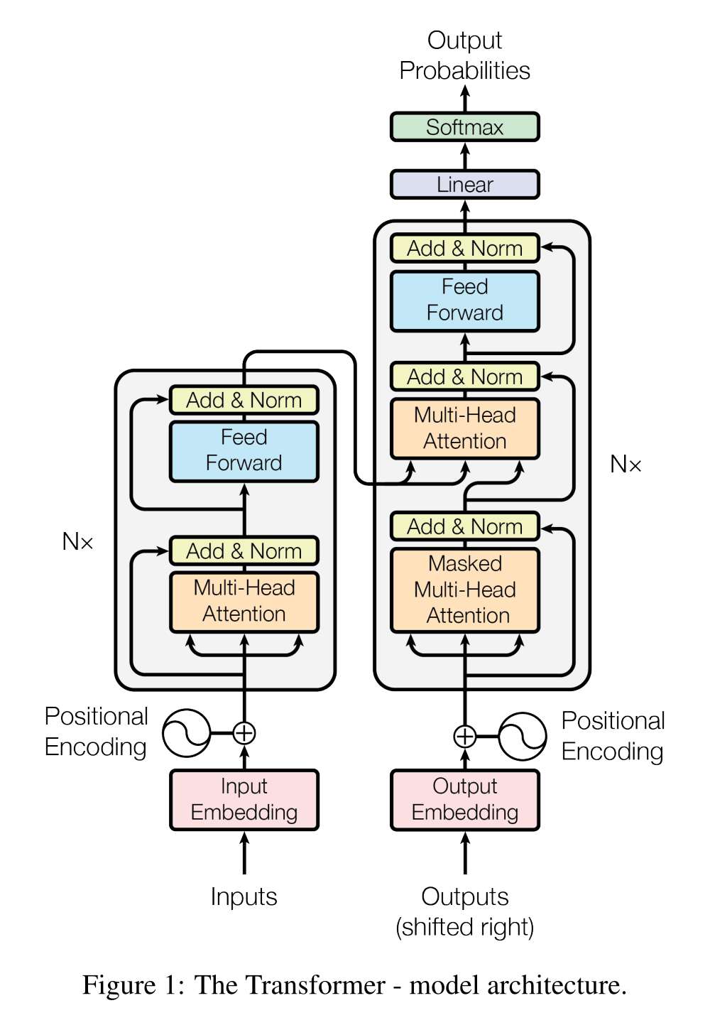
**Figure 2.** Original Transformer architecture. Reproduced from Figure 1 of Vaswani et al. (2017, v7), with the source's scholarly reproduction permission.[^transformer]
**Image description:** Figure 1 from Attention Is All You Need. A repeated encoder stack on the left supplies memory to the repeated decoder stack on the right. The decoder has masked self-attention, cross-attention, and a vocabulary prediction head. Each sublayer is followed by Add and Norm.
The encoder creates contextual representations of a source sequence. The
decoder reads a target prefix and that encoder memory to predict the next
target token. Its masked self-attention prevents access to later target
positions; cross-attention can read all unpadded source positions.
The paper draws **post-normalization**: residual addition comes before LayerNorm.[^transformer]
### Follow the top level contract
**Figure 3.** Two streams connected by encoder memory. Original diagram based on
the Transformer architecture and Harvard implementation.[^transformer][^harvard]
Let `B` be batch size, `S` source length, `T` target input length, `D` model
width, and `V` target vocabulary size. The two sequence lengths can differ:
cross-attention uses `T` queries against `S` keys and values.
| Value | Shape | Meaning |
| --- | --- | --- |
| Source IDs | `B × S` | Source token indices |
| Source embedding | `B × S × D` | Token features plus position |
| Encoder memory Z | `B × S × D` | Contextual source features |
| Shifted target IDs | `B × T` | Target prefix at each position |
| Decoder hidden states | `B × T × D` | Contextual target features |
| Vocabulary logits or log probabilities | `B × T × V` | Next token scores per target position |
This shape ledger is a local derivation from the module interfaces.[^harvard]
The encoder preserves `S`; the decoder preserves `T`; neither requires
source length to equal target length.
About the code examples
These are teaching excerpts, not a standalone runnable library. They assume
PyTorch and the helper modules from the pinned Harvard tutorial. Differences
between the original paper and the tutorial are explained where they matter.
Adapted code is MIT licensed, copyright 2018 Alexander Rush. The
full license notice is retained in
`public/licenses/annotated-transformer-MIT.txt`.[^harvard][^harvard-license]
```python
# Adapted from Harvard NLP, commit debc9fd, MIT license.
class EncoderDecoder(nn.Module):
def __init__(self, encoder, decoder, src_embed, tgt_embed, generator):
super().__init__()
self.encoder, self.decoder = encoder, decoder
self.src_embed, self.tgt_embed = src_embed, tgt_embed
self.generator = generator
def forward(self, src, tgt, src_mask, tgt_mask):
memory = self.encode(src, src_mask)
return self.decode(memory, src_mask, tgt, tgt_mask)
def encode(self, src, src_mask):
return self.encoder(self.src_embed(src), src_mask)
def decode(self, memory, src_mask, tgt, tgt_mask):
return self.decoder(self.tgt_embed(tgt), memory, src_mask, tgt_mask)
```
The top level `forward` returns **decoder features**, not probabilities.
The generator is a separate vocabulary projection followed by log-softmax:
```python
# Adapted from the same pinned Harvard implementation.
class Generator(nn.Module):
def __init__(self, d_model, vocab):
super().__init__()
self.proj = nn.Linear(d_model, vocab)
def forward(self, x):
return F.log_softmax(self.proj(x), dim=-1)
```
`D` is a representation width; `V` is a number of candidate tokens. A modern
loss API may consume raw logits and apply the stable log-softmax internally.
For example, PyTorch CrossEntropyLoss expects unnormalized logits and applies
log-softmax internally. Check the API contract rather than assuming every loss
expects the tutorial’s output.[^crossentropy]
The tutorial’s generator returns log probabilities for its KL loss.[^harvard]
The separate generator also makes weight tying an explicit choice. The original
paper shares embedding and output projection weights; the pinned tutorial
factory instantiates separate modules rather than establishing that sharing.
A shared matrix needs compatible vocabulary and width contracts.[^transformer][^harvard]
## Attention and masking
### One head from scores to content
Queries encode matching features for destination positions. Keys encode matching
features for source positions. Values carry the content to combine. “What I seek,”
“how I can be found,” and “what I carry” are useful interpretations, not fixed
semantic roles assigned to individual neurons.
$$
\operatorname{Attention}(Q,K,V)
=\operatorname{softmax}\left(\frac{QK^\top}{\sqrt{d_k}}\right)V
\tag{1}
$$
Here $d_k$ is key width, and softmax normalizes over key
positions. This is the paper's original scaled dot product attention formula.[^transformer]
When masking is needed, forbidden scores are set to negative infinity before
softmax. Implementations can replace logits or use a fused causal kernel rather
than materializing an additive mask.[^transformer][^sdpa]
**Figure 4.** Scores become weights, then weighted content. Original diagram based
on the paper and Harvard implementation; example numbers are calculated here.[^transformer][^harvard]
Queries and keys determine routing weights; values supply the content to mix.[^transformer]
The grid shows permitted connections, not attention weights. For the illustrated
query 2, scaled scores `[2, 1, 4]` become `[2, 1, −∞]`, giving weights about
`[0.731, 0.269, 0]`. The output is therefore about 0.731 times the first value
vector plus 0.269 times the second. This row is an illustrative calculation,
not a measured model result.
For one head, `Tq` queries and `Tk` key/value positions give:
| Tensor | Shape | Interpretation |
| --- | --- | --- |
| Q | `B × Tq × dₖ` | Destination matching features |
| K | `B × Tk × dₖ` | Source matching features |
| V | `B × Tk × dᵥ` | Source content |
| QKᵀ and attention weights | `B × Tq × Tk` | One routing distribution per query |
| Output | `B × Tq × dᵥ` | Weighted source content |
K and V must share their sequence length because the weight assigned to key `j`
multiplies value `j`. Q can have a different length. The contraction is over key
positions, leaving one output for every query. These shapes follow directly from
the attention equation.[^transformer]
### Why divide by the square root
Under the illustrative assumption that components of q and k are independent,
zero mean, and unit variance:
$$
q^\top k=\sum_{i=1}^{d_k}q_i k_i,
\qquad \operatorname{Var}(q^\top k)=d_k
\tag{2}
$$
The standard deviation grows as $\sqrt{d_k}$. Dividing by that factor keeps the scale
near one under these assumptions and helps avoid saturating softmax early.
This is a variance argument, not a claim that learned features always obey
those assumptions.[^transformer]
```python
# Adapted from Harvard NLP's attention function, MIT license.
def attention(query, key, value, mask=None, dropout=None):
scores = query @ key.transpose(-2, -1)
scores = scores / math.sqrt(query.size(-1))
if mask is not None:
# This teaching variant uses -inf instead of the tutorial's -1e9.
scores = scores.masked_fill(~mask.bool(), float('-inf'))
weights = scores.softmax(dim=-1)
if dropout is not None:
weights = dropout(weights)
return weights @ value, weights
```
The order is score, scale, mask, normalize, optional training dropout, and value
mixing. Softmax produces normalized rows **before** dropout; a realized row after
dropout need not sum to one. Every scored row needs at least one visible key.
An all `−∞` row has no meaningful softmax distribution. The tutorial’s finite
sentinel does not fix that semantic error, and `−1e9` is not safe for every dtype.
This excerpt is for understanding, not a substitute for a tested production kernel.[^harvard]
### Padding and causality are different restrictions
In [Figure 4](#figure-4), multiplying scores by the Boolean mask instead would
give `[2, 1, 0]`, which still assigns positive probability to
the blocked cell. Masking weights afterwards requires explicit renormalization.
This numerical example is a local calculation.
| Mask | What it excludes | Shape before head broadcast |
| --- | --- | --- |
| Source padding | Padded source keys | `B × 1 × S` |
| Target padding | Padded target keys | `B × 1 × T` |
| Causal visibility | Keys later than the query | `1 × T × T` |
| Combined target visibility | Padding or future keys | `B × T × T` |
```python
# Adapted from Harvard NLP's subsequent_mask, MIT license.
def subsequent_mask(length):
future = torch.triu(torch.ones(1, length, length), diagonal=1).bool()
return ~future # True means visible in this page's teaching code.
```
Decoder row $i$ can see keys $j \le i$. This diagonal is valid because the input
is shifted relative to the label. Source padding is reused in encoder
self-attention and decoder cross-attention. Mask polarity differs across APIs:
shape compatibility alone does not establish correct semantics.[^harvard][^sdpa]
### Multi-head attention
Each head uses learned Q, K, and V projections. Its attention weights can differ
from those of another head. The outputs are concatenated and projected back to
model width. Concatenation is not averaging, and projecting into several spaces
is not simply copying the same attention computation.[^transformer]
$$
\begin{aligned}
\operatorname{head}_i
&=\operatorname{Attention}(QW_i^Q,KW_i^K,VW_i^V) \\
\operatorname{MultiHead}(Q,K,V)
&=\operatorname{Concat}(\operatorname{head}_1,\ldots,\operatorname{head}_H)W^O
\end{aligned}
\tag{3}
$$
**Figure 5.** Parallel heads, concatenated outputs. Original diagram based on
the paper and Harvard implementation; head cards are illustrative.[^transformer][^harvard]
Query states have shape `B × Tq × D`; key and value states have shape
`B × Tk × D`. Each head forms `Tq × Tk` attention weights per batch item and
returns `B × Tq × dv`. Concatenation and the output projection restore width `D`.
In self-attention both inputs are the same states; in cross-attention their
sequence lengths can differ.[^transformer][^harvard]
For $H$ heads in the original equal width setup, $d_k=d_v=D/H$:
```text
Learned projections B × T × D
Reshape B × T × H × d
Transpose B × H × T × d
Attention scores B × H × Tq × Tk
Head outputs B × H × Tq × d
Transpose back B × Tq × H × d
Concatenate B × Tq × D
Output projection B × Tq × D
```
```python
# Adapted shape excerpt from Harvard's MultiHeadedAttention, MIT license.
if mask is not None:
mask = mask.unsqueeze(1) # Share visibility across the head axis.
query, key, value = [
linear(x).view(batch_size, -1, num_heads, head_width).transpose(1, 2)
for linear, x in zip(qkv_linears, (query, key, value))
]
head_output, weights = attention(query, key, value, mask=mask)
output = head_output.transpose(1, 2).contiguous().view(
batch_size, -1, num_heads * head_width
)
output = output_linear(output)
```
`transpose` changes strides. The tutorial requests contiguous storage before
using `view` to merge head and feature axes. If using `reshape` instead, understand
when it can copy rather than assume the memory layout stayed unchanged.[^harvard]
### Three attention patterns
| Location | Query input | Key and value input | Visibility |
| --- | --- | --- | --- |
| Encoder self-attention | Source states | Same source states | Unpadded source |
| Decoder self-attention | Target states | Same target states | Unpadded causal prefix |
| Cross-attention | Decoder states | Encoder memory | Unpadded source |
The function is the same; tensor origin and visibility change. This is why
cross-attention can return `T` outputs while reading `S` memory positions.[^transformer]
### MHA, GQA, and MQA
These variants can retain the same query head count `Hq`. What changes is the
number of distinct key and value heads `Hkv`.
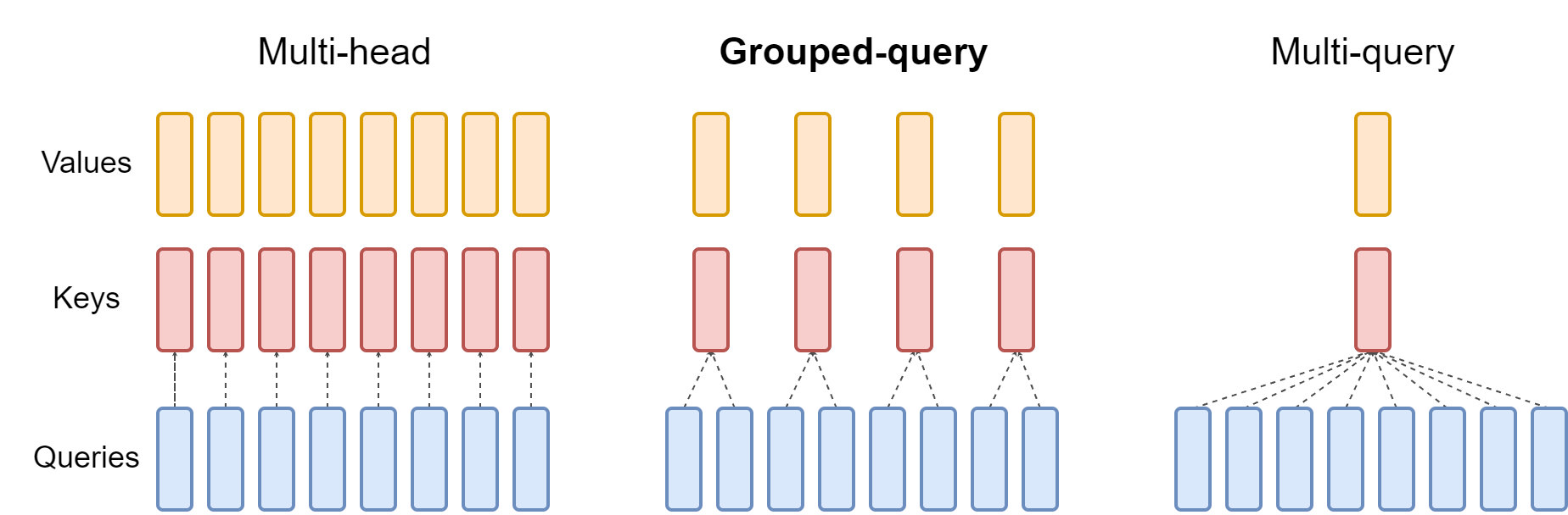
**Figure 6.** Query and KV sharing. Reproduced unchanged from Figure 2 of Ainslie et al., GQA (2023), under CC BY 4.0.[^gqa]
**Image description:** Figure 2 from the GQA paper. Eight query heads each have separate KV heads in MHA, share KV heads in pairs in GQA, and all share one KV head in MQA.
| Variant with Hq = 8 | Hkv | KV sharing | Relative cache elements |
| --- | ---: | --- | ---: |
| MHA | 8 | One KV pair per query head | 100% |
| Illustrated GQA | 4 | Two query heads per KV pair | 50% |
| MQA | 1 | All query heads share one KV pair | 12.5% |
Each query head still produces its own score matrix and weighted output. Q has
shape `B × Hq × Tq × dₖ`, K has `B × Hkv × Tk × dₖ`, and V has
`B × Hkv × Tk × dᵥ`. A mapping $g(h)$ assigns each query head its KV head:
$$
\operatorname{head}_h
=\operatorname{softmax}\left(\frac{Q_h K_{g(h)}^\top}{\sqrt{d_k}}\right)V_{g(h)}
\tag{4}
$$
For equal groups, each KV head serves `Hq/Hkv` query heads. Efficient kernels
can reuse K/V without materializing copies for every query head.[^sdpa] The table’s cache
fractions are a local derivation for equal head width and sequence length.[^gqa]
The GQA paper also converts MHA checkpoints by averaging groups of K/V projection
heads and continuing training. That is an **uptraining recipe**, not a pooling
operation in every GQA forward pass. KV sharing primarily targets cache and
memory bandwidth; it does not turn full attention into a linear operator.[^gqa]
## Components and full model
### The assembly map
**Figure 7.** Residual bypasses and repeated layers. Original diagram of the
pinned Harvard Pre-LN implementation, not the paper's Post-LN order.[^harvard][^transformer]
Each sublayer transforms a normalized branch; its unchanged input bypasses that
branch and is added back after dropout. An encoder layer has self-attention and
FFN blocks; a decoder layer adds cross-attention. Each stack repeats its layer
`N` times with independent parameters, then applies a final LayerNorm.[^harvard]
### Residual paths and normalization
The Harvard wrapper normalizes the input before the sublayer:
$$
\begin{aligned}
\text{Pre-LN:}\quad y
&=x+\operatorname{Dropout}\bigl(F(\operatorname{LN}(x))\bigr) \\
\text{Post-LN:}\quad y
&=\operatorname{LN}\bigl(x+\operatorname{Dropout}(F(x))\bigr)
\end{aligned}
\tag{5}
$$
```python
# Adapted from Harvard NLP's SublayerConnection, MIT license.
class SublayerConnection(nn.Module):
def __init__(self, size, dropout):
super().__init__()
self.norm = LayerNorm(size)
self.dropout = nn.Dropout(dropout)
def forward(self, x, sublayer):
return x + self.dropout(sublayer(self.norm(x)))
```
Residual addition requires matching shapes. It carries the input forward while
adding a learned update. LayerNorm transforms each token’s feature vector without
mixing sequence positions. Normalization placement changes the gradient path;
it is not merely interchangeable notation. The tutorial additionally normalizes
the output of each completed stack.[^harvard][^preln]
Read the implementation as well as the name. The pinned tutorial’s custom
LayerNorm uses `x.std` and adds epsilon outside the standard deviation. That
does not establish numerical equivalence to a framework LayerNorm with its
own variance estimator and epsilon convention. For a reproduction, preserve
the implementation; for new code, use a tested layer and document the change.[^harvard]
### Encoder and decoder layers
```python
# Explanatory pseudocode adapted from the pinned Harvard layers.
def encoder_layer(x, source_mask):
x = residual(x, lambda h: self_attention(h, h, h, source_mask))
return residual(x, feed_forward)
def decoder_layer(x, memory, source_mask, target_mask):
x = residual(x, lambda h: self_attention(h, h, h, target_mask))
x = residual(x, lambda h: cross_attention(h, memory, memory, source_mask))
return residual(x, feed_forward)
```
The wrapper passes normalized `h` to the lambda. In cross-attention, only the
decoder query stream follows that residual wrapper; keys and values come from
the already encoded memory. The self-attention and cross-attention objects
have separate learned projection weights.[^harvard]
### The position wise FFN
$$
\operatorname{FFN}(x)=\operatorname{ReLU}(xW_1+b_1)W_2+b_2
\tag{6}
$$
Attention determines which contextual information reaches a position. The FFN
then provides a nonlinear feature transformation at that position, using shared
weights across tokens. It does not directly mix the sequence axis. The paper’s
base configuration expands width `512 → 2048 → 512`.[^transformer]
```python
# Adapted from Harvard's PositionwiseFeedForward, MIT license.
def forward(self, x):
return self.w_2(self.dropout(self.w_1(x).relu()))
```
The expansion gives the nonlinear operation more intermediate features while
the contraction restores the residual interface. Without an intervening
nonlinearity, two linear transformations would collapse into one linear map.
That is an algebraic explanation, not proof that every expansion ratio is optimal.
### Embeddings and sinusoidal position
Token IDs select learned vectors. The tutorial multiplies them by $\sqrt{D}$, adds
a sinusoidal position vector, then applies dropout:
$$
\begin{aligned}
\operatorname{PE}(p,2i)&=\sin\left(\frac{p}{10000^{2i/D}}\right) \\
\operatorname{PE}(p,2i+1)&=\cos\left(\frac{p}{10000^{2i/D}}\right)
\end{aligned}
\tag{7}
$$
Each sine and cosine pair uses a different angular frequency. The position
vector has width `D` so it can be added to token features; a stored
`1 × max_length × D` buffer broadcasts across the batch.[^transformer][^harvard]
**Figure 8.** Position at different frequencies. Calculated from the paper's
sinusoidal rule for a toy width of `D = 8`.[^transformer]
Three channel pairs are plotted over positions 0–63, with angular frequencies
`1`, `0.1`, and `0.01`. The fourth pair, at `0.001`, is omitted. Every pair has
a sine channel starting at zero and a cosine channel starting at one; lower
frequencies vary more slowly. The lines show the analytical functions between
integer positions, not a measured model result.
```python
# Teaching excerpt adapted from Harvard, MIT license; D is even here.
positions = torch.arange(max_length).unsqueeze(1)
frequencies = torch.exp(torch.arange(0, D, 2) * (-math.log(10000.0) / D))
pe = torch.zeros(max_length, D)
pe[:, 0::2] = torch.sin(positions * frequencies)
pe[:, 1::2] = torch.cos(positions * frequencies)
# In an nn.Module, register the fixed tensor as a buffer, not a parameter.
self.register_buffer('pe', pe.unsqueeze(0))
model_input = dropout(embedding(token_ids) * math.sqrt(D) + self.pe[:, :T])
```
Sine and cosine addition identities make a fixed position offset a linear
rotation within each pair. This explains the relative offset motivation; it
does not guarantee useful generation beyond the trained length. Ordinary
self-attention alone, without position or asymmetric visibility, cannot
distinguish arbitrary permutations by order.[^transformer]
### Independent layers and the factory
Deep-copying a module creates independent parameter objects. Calling the same
module object N times ties weights. Identical structure and identical initial
values are not the same as shared parameters. The tutorial factory builds
distinct encoder/decoder layers and distinct self/cross-attention modules:
```python
# Condensed from Harvard's make_model; classes come from that tutorial.
c = copy.deepcopy
attn = MultiHeadedAttention(heads, d_model)
ff = PositionwiseFeedForward(d_model, d_ff, dropout)
position = PositionalEncoding(d_model, dropout)
model = EncoderDecoder(
Encoder(EncoderLayer(d_model, c(attn), c(ff), dropout), layers),
Decoder(DecoderLayer(d_model, c(attn), c(attn), c(ff), dropout), layers),
nn.Sequential(Embeddings(d_model, source_vocab), c(position)),
nn.Sequential(Embeddings(d_model, target_vocab), c(position)),
Generator(d_model, target_vocab),
)
for parameter in model.parameters():
if parameter.dim() > 1:
nn.init.xavier_uniform_(parameter)
```
The factory’s Xavier initialization follows construction. Architecture
contracts alone do not specify optimization behavior.[^harvard]
| Boundary | Invariant |
| --- | --- |
| Embedding to stack | Final width D |
| Sublayer to residual add | Same input and output shape |
| Original head split | D divisible by H |
| Memory to cross-attention | Width compatible with K/V projections |
| Decoder to generator | Width D |
| Generator to loss | Vocabulary axis V and correctly aligned labels |
This boundary checklist is a local synthesis of the paper and tutorial
interfaces.[^transformer][^harvard]
## Training and inference
### Teacher forcing and shifted labels
**Figure 9.** Parallel training, autoregressive generation. Original diagram
based on Harvard's Batch and decoding loops; EOS stopping is added here.[^harvard]
During training, shifted inputs are known in advance and scores at each position
are compared with the next known label. Labels enter the loss, not a token
selection step. During generation, the selected token is appended to the prefix
and fed back for the next step; stop at EOS or the length limit. Cache reuse
changes the work performed, not this dependency.[^harvard][^generation][^cache]
```text
Full target BOS y₁ y₂ y₃ EOS
Decoder input BOS y₁ y₂ y₃
Prediction label y₁ y₂ y₃ EOS
```
All correct previous tokens are available at training time. The causal mask
prevents a prediction from reading future target inputs. Teacher forcing does
not mean that future labels are visible through attention. At inference time
the model conditions on its own previous choices instead.[^harvard]
```python
# Condensed from Harvard's Batch, MIT license.
source_mask = (source != pad_id).unsqueeze(-2)
target_input = target[:, :-1]
target_label = target[:, 1:]
target_mask = (target_input != pad_id).unsqueeze(-2)
target_mask = target_mask & subsequent_mask(target_input.size(-1)).to(target.device)
token_count = (target_label != pad_id).sum()
```
Padding masks block padded keys; loss handling separately excludes padded
prediction targets. Padded query rows can still produce hidden states, which
must not accidentally become supervised targets. Normalize the loss by actual
targets, not the padded area of the batch.[^harvard]
### Forward pass and optimization
A training step prepares inputs and masks, runs the model and generator,
computes token loss, normalizes it, backpropagates, updates parameters at the
chosen optimizer boundary, advances the scheduler, and clears gradients.
Evaluation disables parameter updates and training dropout. Architecture
defines the differentiable function; the loop defines execution policy.[^harvard]
The paper used Adam with $\beta_1=0.9$, $\beta_2=0.98$, and $\epsilon=10^{-9}$, and a warmup followed
by inverse square root decay. These are historical recipe choices, not defaults
recommended for every current model.[^transformer]
$$
\operatorname{lr}(s)=\text{factor}\cdot D^{-1/2}
\min\left(s^{-1/2},s\,w^{-3/2}\right)
\tag{8}
$$
Here $s$ is optimizer step and $w$ is warmup length. Before $w$ the schedule
rises linearly; at $w$ the branches meet; afterwards it decays as $s^{-1/2}$.
The tutorial exposes a multiplicative `factor`:[^harvard]
```python
# Adapted from Harvard's rate function, MIT license.
def rate(step, model_size, factor, warmup):
step = max(step, 1)
return factor * model_size ** (-0.5) * min(
step ** (-0.5), step * warmup ** (-1.5)
)
```
### Label smoothing and loss interpretation
For a simplified vocabulary with no padding class, distribute target mass as:
$$
q(y)=1-\epsilon,\qquad
q(k)=\frac{\epsilon}{V-1}\quad\text{for }k\ne y
\tag{9}
$$
The pinned tutorial reserves a padding class, distributes smoothing over $V-2$
alternative classes, sets padding probability to zero, and removes entire loss
rows whose target is padding. It minimizes $\operatorname{KL}(q\Vert p)$ using model log
probabilities as input.[^harvard]
Smoothing discourages assigning all probability to the observed label, but
does not universally improve every metric. The original paper reports improved
accuracy and BLEU while perplexity worsened.[^transformer]
**A useful algebraic distinction:** cross entropy equals $H(q)+\operatorname{KL}(q\Vert p)$.
For a nondegenerate smoothed target, its minimum is positive $H(q)$. KL itself
can reach zero when $p=q$. Do not compare raw smoothed loss to ordinary hard
target cross-entropy as if their baselines were the same.
### The bridge to VLM supervised fine tuning
The same conditional next token objective applies when context $x$ includes
an image and instruction, and $y$ is the target answer:
$$
\mathcal{L}(\theta)
=-\frac{\sum_t m_t\log p_\theta(y_t\mid x,y_{\lt t})}{\sum_t m_t}
\tag{10}
$$
Here $y_{\lt t}$ denotes the preceding answer tokens, and $m_t$ selects supervised
positions with at least one selected target. This is local notation for token
averaged conditional cross-entropy, with the conditional objective and ignore rules described by SFT and loss
documentation. It is not a proprietary training recipe.[^sft][^crossentropy]
An **attention mask** controls what a position can read. A **loss mask** controls
which predictions contribute gradients. Prompt tokens can remain visible
context while their prediction targets are ignored. Completion or assistant
only loss depends on data format, chat template, and configuration. Inspect
decoded examples and labels rather than relying on a setting’s name.[^sft]
With $b$ examples per device, $a$ accumulated microbatches, and $n$ data parallel
workers, the nominal effective batch is $b\cdot a\cdot n$. That count does not prove
numerical equivalence to one physical batch.
For microbatch $j$ with summed token loss $S_j$ and supervised token count $N_j$,
the true combined token mean is:
$$
\overline{\mathcal{L}}_{\text{tokens}}=\frac{\sum_j S_j}{\sum_j N_j}
\tag{11}
$$
It is not generally the mean of $S_j/N_j$. For example, token means 1 and 3 over
10 and 30 tokens give a combined mean 2.5, not 2. Choose whether tokens or
examples should receive equal weight, and make distributed reductions and
gradient scaling implement that choice. This is a local derivation.
Mixed precision scaling, clipping, and optimizer stepping must respect the
effective batch boundary.[^amp]
Full fine tuning updates the selected model weights. LoRA freezes base weights
and learns low rank updates to selected matrices. It reduces trainable
parameters and their optimizer state, not the need to run the base model.
Rank and target matrices are design choices; fewer trainable parameters do
not automatically mean a smaller inference model.[^lora]
### Evaluate a data or training change
This is a proposed experiment checklist, not a report of executed experiments:
1. Define the hypothesis, downstream metric, and important workload slices.
2. Separate training, development, and final test roles. Group pages and
synthetic variants of one source document when a random split would leak
shared information. Hold out templates or sources if that is the intended
generalization test.
3. Fix the starting checkpoint, evaluation protocol, and declared budget.
Equal steps and equal tokens are different comparisons.
4. For two changes, compare baseline, A, B, and A+B when feasible.
5. Repeat training when feasible. Resampling evaluation documents does not
measure training seed variability.
6. If only A+B was tested, attribute the result to that combined intervention.
### Greedy decoding and the cache
```python
# Condensed from Harvard's greedy_decode, MIT license.
# Assumes one source example. No KV cache is implemented in this excerpt.
memory = model.encode(source, source_mask)
prefix = torch.tensor([[bos_id]], device=source.device)
for _ in range(max_length - 1):
mask = subsequent_mask(prefix.size(1)).to(source.device)
hidden = model.decode(memory, source_mask, prefix, mask)
log_probs = model.generator(hidden[:, -1])
next_token = log_probs.argmax(dim=-1)
prefix = torch.cat([prefix, next_token[:, None]], dim=1)
# Added stopping rule; the pinned tutorial runs to the length limit.
if next_token.item() == eos_id:
break
```
Use evaluation mode and disable gradient recording for generation. The
tutorial’s simple loop recomputes the full prefix each step; source memory is
computed once. The EOS break above is an explicit teaching addition.[^harvard]
Incremental causal decoding can instead reuse each layer’s earlier K/V. The
new query reads cached history plus its own new K/V. Earlier causal states do
not change when a later token is appended, so reuse preserves the model’s
causal computation, up to numerical differences. For encoder/decoder models,
cross-attention K/V derived from fixed memory can also be reused.[^cache]
For $L$ layers, cached length $T_{\text{cache}}$, equal key/value head width $d$, and
$s$ bytes per element, a simple uncompressed self attention cache uses:
$$
\text{KV cache bytes}\approx 2LB\,T_{\text{cache}}H_{\text{kv}}d\,s
\tag{12}
$$
This is a local element-count derivation. It excludes allocation overhead,
padding, sharding, quantization metadata, and any extra cross-attention cache.
For unequal K/V widths, replace $2d$ with $d_k+d_v$.
Greedy decoding selects the most probable next token locally. Beam search
retains candidate prefixes; temperature rescales logits; top-k truncates to a
fixed number of candidates; nucleus sampling retains a probability mass.
These are decoding policies, not different trained architectures. Their
usefulness depends on the task; greedy choice does not guarantee the best
whole sequence.[^generation][^nucleus]
### Computational cost
For a dense decoder with $L$ layers, batch $B$, sequence length $T$, width $D$,
and FFN width proportional to $D$, a local matrix multiplication count gives:
Full sequence forward:
$$
\mathcal{O}\bigl(LB(TD^2+T^2D)\bigr)
\tag{13}
$$
One cached decoding step at history length $T$:
$$
\mathcal{O}\bigl(LB(D^2+TD)\bigr)
\tag{14}
$$
Projections and the FFN contribute the width squared term; $QK^\top$ and weight/value
mixing contribute the sequence interaction term. This omits the vocabulary
head, whose full sequence cost can be $\mathcal{O}(BTDV)$, and assumes ordinary dense
attention rather than experts or restricted connectivity. A causal triangle
changes constants, not quadratic growth. A full sequence forward is not the
cost of repeatedly recomputing that prefix during generation.
The attention score tensor contains $BHT^2$ elements if materialized. Exact tiled
kernels can avoid storing that full matrix while retaining quadratic arithmetic.[^flashattention]
## From Transformer to modern LLMs
**Figure 10.** Coexisting design choices, not an inevitable timeline. Original
comparison synthesized from the cited architecture and implementation sources.[^transformer][^gpt2][^rmsnorm][^rope][^swiglu][^gqa][^flashattention][^cache]
### One causal stream instead of two
A decoder language model removes the separate source encoder and its
cross-attention path. Prompt, context, and continuation occupy one causal
sequence. Attention, FFN, residual width, normalization, position, and a
vocabulary head remain recognizable. GPT-2 is a concrete example with learned
position embeddings and pre-normalized blocks, not the full list of later
choices in the diagram.[^gpt2]
### LayerNorm and RMSNorm
LayerNorm centers a feature vector and rescales it using variance. RMSNorm
rescales by root mean square without subtracting the mean. This removes a
statistical operation while preserving rescaling invariance; it is not the same
function as LayerNorm and is not universally better for every model.[^rmsnorm]
### Additive position and RoPE
Sinusoidal position adds a vector to the input residual stream. RoPE instead
rotates query and key feature pairs with position dependent angles, making
their dot product depend on relative displacement. It changes compatibility
geometry, not just a stored table. Reliable long context behavior still needs
appropriate training and evaluation.[^rope]
Continue with [Position and long context](/architectures/evolution/position-and-long-context/).
### ReLU, GELU, and gated FFNs
The original FFN uses ReLU; GPT-2 uses GELU. A gated FFN introduces a second input
projection and multiplies the branches before projecting back:
$$
\begin{aligned}
\operatorname{SwiGLU}(x)&=\bigl[\operatorname{SiLU}(xW_g)\odot(xW_u)\bigr]W_d \\
\operatorname{SiLU}(z)&=z\,\operatorname{sigmoid}(z)
\end{aligned}
\tag{15}
$$
Biases are omitted in this notation. The gate is a learned multiplicative
feature interaction, not a probability constrained to `[0,1]`. SwiGLU uses
three projection matrices, so fair comparisons should account for parameter
and compute budgets, not simply reuse the same hidden width. Shazeer’s paper
reports gains in its controlled experiments, not a universal guarantee.[^swiglu]
Continue with [FFNs and experts](/architectures/evolution/ffns-and-experts/).
### Different meanings of efficient attention
| Change | What changes | What not to infer |
| --- | --- | --- |
| FlashAttention | IO schedule and score materialization | Full attention becomes linear arithmetic |
| MQA or GQA | Distinct KV projection heads and cache | Query head count must shrink |
| Sliding window | Allowed direct connections | Every token still directly reads all history |
| MLA | Joint compressed KV representation | It is just fewer ordinary KV heads |
FlashAttention preserves the dense attention operator up to numerical
differences. Sliding window attention changes connectivity; Mistral describes
how information can still travel across layers. DeepSeek-V2’s MLA introduces
low rank KV compression. These mechanisms address different costs and should
not be bundled into one unexplained claim of efficiency. The comparison table
is a local synthesis of these mechanisms and the GQA design.[^flashattention][^gqa][^mistral][^deepseekv2]
Continue with [Attention and memory](/architectures/evolution/attention-and-memory/).
### Dense and routed experts
An MoE layer routes each token to selected FFN experts rather than activating
all experts. Switch Transformer uses one expert per token with routing weights,
capacity handling, and load balancing. The residual output still has width D.
More total parameters do not imply that all parameters are active for every
token, nor that device communication becomes free.[^switch]
Sparse expert activation is not the same as sparse attention.[^switch]
### Information across depth
Attention and FFNs describe computation within a layer. Residual paths describe
how representations reach later layers. Start with the original single-stream
residual, then compare multiple streams, attention across earlier layers and
gated reads and writes in [Depth and residual paths](/architectures/evolution/depth-and-residual-paths/).
That companion page supplies the equations, source reports and their limits.
### Read a model as a set of contracts
For any model report or implementation, record:
1. Stack: encoder/decoder, prefix, or causal decoder?
2. Normalization: which statistic, and where in the residual path?
3. Position: additive, rotary, learned, or biased?
4. Attention: full, local, latent, linear, or hybrid?
5. Heads: query count, KV count, and head widths?
6. FFN: activation, intermediate width, dense or routed?
7. Context: trained length, served length, and any extension method?
8. Runtime: cache, kernel, precision, and parallelism?
9. Depth: one residual stream, multiple streams, or selective depth reads?
10. Evidence: exact checkpoint, pinned code, and supporting ablations?
This is a local reading checklist. It helps separate the mathematical model
from the strategy used to execute it. For VLMs, add how image features enter
the model and how their positions and token budget are defined.
Continue with [Multimodal integration](/architectures/evolution/multimodal-integration/)
and [Model Deep Dives](/architectures/models/).
## Check your understanding
Shape and information checks
- Why can S differ from T? Cross-attention maps T queries over S keys/values.
- What does the decoder return? D-wide features, before the V-wide generator.
- Which axis does attention softmax normalize? Key positions, for each query.
- Does a causal mask make dense attention linear? No; the dense interaction
matrix remains quadratic in length.
- Does deep-copying layers share parameters? No; reusing the same object would.
- Can ignored prompt labels remain visible context? Yes; loss and attention
masks serve different purposes.[^sft]
- Does KV caching alter causal dependencies? No; it reuses earlier computation.[^cache]
- Does an MoE layer activate every expert? No; the router chooses a subset.[^switch]
Optional implementation checks
1. Assert the source, memory, target, head, residual, and vocabulary shapes.
Deliberately swap sequence axes and predict the first failing operation.
2. Test self-attention, cross-attention with different lengths, padding, and
causality. Changing hidden K/V positions should not change visible outputs
when dropout is disabled.
3. Verify that two cloned layers have distinct parameter storage. Check every
residual addition for equal shapes.
4. Print shifted inputs, labels, and one combined mask row. Compare cached and
uncached generation logits within numerical tolerance.
5. Fill the reading checklist for one model, cite each source section, and mark
whether an efficiency choice changes arithmetic, traffic, cache, or active
parameters.
These are learning exercises, not tests reported as completed on this page.
## Sources and attribution
The primary implementation reference is Harvard NLP’s Annotated Transformer
at commit `debc9fd`.[^harvard] Read the
[original tutorial](https://nlp.seas.harvard.edu/annotated-transformer/)
for its full runnable implementation and experiments. Adapted excerpts retain
Alexander Rush’s MIT license.[^harvard-license] Paper figures retain their own
reproduction terms, not Latent Light’s MIT grant. Numbered references connect
the explanations to their supporting sources.
[^transformer]: Ashish Vaswani et al., [Attention Is All You Need](https://arxiv.org/html/1706.03762v7), NeurIPS 2017, arXiv version 7. Sections 3.1–3.5 define the architecture, attention, FFN, embeddings, and position; sections 5.3–5.4 describe optimization and smoothing. Figure 1 is reproduced under the source's stated scholarly or journalistic reproduction permission.
[^harvard]: Harvard NLP, [The Annotated Transformer](https://github.com/harvardnlp/annotated-transformer/blob/debc9fd747bb2123160a98046ad1c2d4da44a567/the_annotated_transformer.py), commit `debc9fd747bb2123160a98046ad1c2d4da44a567`. Inspected interfaces include EncoderDecoder and Generator (lines 230–269), residuals and stacks (292–438), attention and heads (441–628), FFN and position (677–786), make_model (822–848), Batch and training (907–1024), LabelSmoothing (1148–1176), and greedy_decode (1313–1328). Teaching changes are marked beside the excerpts.
[^harvard-license]: Alexander Rush, [Annotated Transformer MIT license](https://github.com/harvardnlp/annotated-transformer/blob/debc9fd747bb2123160a98046ad1c2d4da44a567/LICENSE), copyright 2018, same pinned commit. The complete notice is retained with the adapted excerpts.
[^scaling-laws]: Jared Kaplan et al., [Scaling Laws for Neural Language Models](https://arxiv.org/abs/2001.08361v1), 2020, arXiv version 1. The authors report empirical relationships between language modeling loss, model size, dataset size, and training compute within the studied ranges. These findings do not guarantee improvement on every downstream task.
[^t5]: Colin Raffel et al., [Exploring the Limits of Transfer Learning with a Unified Text-to-Text Transformer](https://arxiv.org/abs/1910.10683v4), JMLR 2020, arXiv version 4. A shared text input and text output formulation covers translation, summarization, question answering, classification, and other language tasks.
[^pix2seq]: Ting Chen et al., [Pix2seq: A Language Modeling Framework for Object Detection](https://arxiv.org/html/2109.10852v2), ICLR 2022, arXiv version 2. Sections 2.1–2.2 describe serializing object labels and bounding box coordinates into tokens and generating them conditioned on an image.
[^gqa]: Joshua Ainslie et al., [GQA: Training Generalized Multi-Query Transformer Models from Multi-Head Checkpoints](https://aclanthology.org/2023.emnlp-main.298/), EMNLP 2023. Section 2 describes KV sharing and uptraining; Figure 2 compares MHA, GQA, and MQA. The inspected [arXiv HTML version 3](https://arxiv.org/html/2305.13245v3#S2) provides the same mechanism. Figure 2 is reproduced unchanged under CC BY 4.0.
[^preln]: Ruibin Xiong et al., [On Layer Normalization in the Transformer Architecture](https://proceedings.mlr.press/v119/xiong20b.html), ICML 2020. Analysis of normalization placement and gradient behavior.
[^sft]: Hugging Face, [TRL SFT Trainer: completion and assistant message loss](https://huggingface.co/docs/trl/sft_trainer#train-on-assistant-messages-only), inspected October 3, 2026. Configuration and templates determine which tokens are supervised; behavior must be checked against the installed version.
[^amp]: PyTorch, [Automatic mixed precision examples: gradient accumulation](https://docs.pytorch.org/docs/2.14/notes/amp_examples.html#gradient-accumulation), version 2.14. Scaling, clipping, and optimizer boundaries for an effective batch.
[^lora]: Edward J. Hu et al., [LoRA: Low-Rank Adaptation of Large Language Models](https://arxiv.org/abs/2106.09685), 2021, ICLR 2022. Frozen base weights and trainable low rank adaptation matrices.
[^nucleus]: Ari Holtzman et al., [The Curious Case of Neural Text Degeneration](https://arxiv.org/abs/1904.09751), ICLR 2020. Nucleus sampling and comparison with other decoding policies.
[^flashattention]: Tri Dao et al., [FlashAttention: Fast and Memory-Efficient Exact Attention with IO-Awareness](https://arxiv.org/html/2205.14135v2#S3), NeurIPS 2022, arXiv version 2. Sections 2–3 distinguish attention arithmetic from memory traffic and materialization.
[^gpt2]: Alec Radford et al., OpenAI, [Language Models are Unsupervised Multitask Learners](https://cdn.openai.com/better-language-models/language_models_are_unsupervised_multitask_learners.pdf), 2019, section 2.3. GPT-2 architecture and normalization changes.
[^rmsnorm]: Biao Zhang and Rico Sennrich, [Root Mean Square Layer Normalization](https://arxiv.org/abs/1910.07467), NeurIPS 2019. Rescaling without mean centering.
[^rope]: Jianlin Su et al., [RoFormer: Enhanced Transformer with Rotary Position Embedding](https://arxiv.org/html/2104.09864v5#S3), 2021, arXiv version 5, section 3. Position dependent rotations and relative displacement in query/key dot products.
[^swiglu]: Noam Shazeer, [GLU Variants Improve Transformer](https://arxiv.org/html/2002.05202v1), 2020, arXiv version 1. Gated FFN definitions and controlled comparisons.
[^mistral]: Albert Q. Jiang et al., [Mistral 7B](https://arxiv.org/html/2310.06825v1#S2), 2023, arXiv version 1, section 2. Sliding window connectivity and information propagation across layers.
[^deepseekv2]: DeepSeek-AI, [DeepSeek-V2: A Strong, Economical, and Efficient Mixture-of-Experts Language Model](https://arxiv.org/html/2405.04434v5#S2.SS1), 2024, arXiv version 5, section 2.1. Multi-head latent attention and joint KV compression.
[^switch]: William Fedus, Barret Zoph, and Noam Shazeer, [Switch Transformers: Scaling to Trillion Parameter Models with Simple and Efficient Sparsity](https://arxiv.org/html/2101.03961v3#S2), JMLR 2022, arXiv version 3, sections 2–3. Expert routing, capacity, and balancing.
[^sdpa]: PyTorch, [Scaled dot product attention](https://docs.pytorch.org/docs/2.14/generated/torch.nn.functional.scaled_dot_product_attention.html), version 2.14. Mask polarity, causal handling, backend selection, GQA, and numerical differences between kernels.
[^crossentropy]: PyTorch, [CrossEntropyLoss](https://docs.pytorch.org/docs/2.14/generated/torch.nn.CrossEntropyLoss.html), version 2.14. Logit inputs, LogSoftmax equivalence, ignored labels, and loss reduction.
[^cache]: Hugging Face, [Transformers cache strategies](https://huggingface.co/docs/transformers/main/en/kv_cache), main documentation inspected October 3, 2026. KV reuse and the encoder/decoder cache section. Main documentation can change; check the installed version when implementing.
[^generation]: Hugging Face, [Transformers GenerationConfig](https://huggingface.co/docs/transformers/main/en/main_classes/text_generation#transformers.GenerationConfig), main documentation inspected October 3, 2026. Greedy decoding, beams, temperature, top-k, and top-p parameters.
Source: https://latentlit.com/architectures/foundations/index.mdx