---
title: "Hardware 101 for AI Researchers and Engineers"
description: "A foundation for building AI devices, from electricity and sensors to processors, memory, embedded software, power and practical measurement."
---
> Documentation Index
> Fetch the complete documentation index at: https://latentlit.com/llms.txt
> Use this file to discover all available pages before exploring further.
# Hardware 101 for AI Researchers and Engineers
import FocusCanvas from '../../../components/FocusCanvas.astro';
import SourceFigure from '../../../components/architectures/SourceFigure.astro';
import HardwareFigure from '../../../components/hardware/HardwareFigure.astro';
import HardwareBudget from '../../../components/hardware/HardwareBudget.astro';
import ComparisonTable from '../../../components/ComparisonTable.astro';
Full stack often means connecting the frontend and backend of a software
product. For AI device builders, I think the next full stack brings together
**AI + software + hardware**.
Imagine a small assistant that can hear a request, recognize an object and
respond. A model supplies the learned capability. Software moves data and
coordinates behavior. Hardware captures signals, runs computation and produces
the response within limits of memory, timing, energy and heat. Each layer
changes what the others can do.
That is the ambition behind this tutorial: **learn across the stack to turn an
AI idea into a useful device**. Hardware foundations give us a way to understand
those connections, ask better design questions and start building.
[Figure 1](#figure-1) previews the learning journey and what you can do with it.
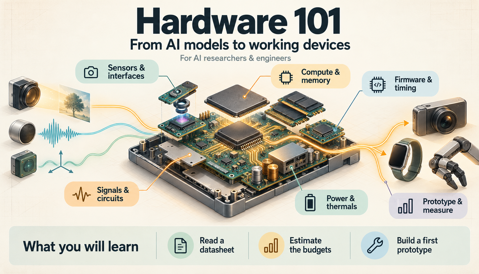
**Figure 1.** From AI models to working devices: the tutorial at a glance. Moving lights suggest information flowing from sensors through computation to outputs; their timing is illustrative. AI-generated learning map and keyframe, with an assembled animation, informed by signal acquisition, chip integration and device power constraints; the hardware illustrations are schematic.[^sampling][^board][^buck]
**Image description:** Hardware 101: from AI models to working devices. Six learning areas connect a conceptual AI-device workbench: signals and circuits, sensors and interfaces, compute and memory, firmware and timing, power and thermals, and prototyping and measurement. The learning outcomes are to read a datasheet, estimate the budgets and build a first prototype. Camera, microphone, motion-sensor, wearable and robotic-gripper illustrations suggest several device types; they are not a literal circuit or measured system.
[Open animated GIF](/figures/hardware/hardware-101-learning-map-motion-v1.gif)
Read the learning map
- **Signals and circuits:** understand voltage, current, logic levels and the physical meaning of a bit.
- **Sensors and interfaces:** turn physical observations into useful samples and move them through the device.
- **Compute and memory:** understand execution engines, working sets, storage and data movement.
- **Firmware and timing:** coordinate peripherals, buffers and model execution within the required response time.
- **Power and thermals:** estimate energy needs and distinguish average consumption from peak and sustained limits.
- **Prototype and measure:** read the hardware contract, bring up one layer at a time and test the complete path.
The practical goal is to **read a datasheet, estimate the budgets and build a
first prototype**, using the same foundations across different kinds of AI device.
This is a foundation for learning to build those systems. It assumes you can
write software and understand what a model does, while introducing hardware
from first principles. The goal is to read a block diagram, understand a
datasheet, estimate the important budgets and begin a measured prototype.
The examples span several device types because the foundations transfer.
Start with [electricity and signals](#electricity-and-digital-signals), then
[processors](#understand-the-chip) and [memory](#memory-is-a-working-material).
Continue through [interfaces](#connect-the-parts), [embedded software](#software-owns-time)
and [power](#power-heat-and-the-physical-device). The [budget lab](#three-budgets-you-can-change),
[prototype workflow](#read-the-contract-then-build) and [2026 platform map](#a-small-platform-map-for-2026)
turn the concepts into practical questions.
## See the whole device
A good first drawing has two paths: **what happens to the information**, and
**where the energy goes**. Add the clocks, software and feedback that coordinate
them. [Figure 2](#figure-2) gives us this view before we zoom into individual parts.
**Follow information. Follow energy. Follow control.**
An AI device joins a physical world to a computing system.
**Information:** Sense → Buffer → Compute → Decide → Act. Light, sound or motion → samples and timestamps → model inputs → a decision → a display, speaker or actuator.
**Energy:** Source → Convert → Distribute → Use → Dissipate. Battery or supply → regulators → power rails → sensors, compute, radios and outputs → heat and useful physical work.
**Control:** Boot → Configure → Schedule → Observe → Recover. Clocks and reset establish a start; firmware coordinates work, checks deadlines and handles failures. Feedback returns through sensing.
**Five scales:**
1. **Component:** A resistor, sensor or regulator.
2. **Chip:** Cores, memory and peripherals.
3. **Board:** Connections, rails and connectors.
4. **Device:** Enclosure, battery and interaction.
5. **System:** Devices, networks and services.
These are views of one design, not three independent pipelines or a literal wiring diagram. A chip is itself a component at board scale.
**Figure 2.** Three flows through an AI device, viewed at five scales. Original synthesis informed by sampled-data systems, MCU integration and heterogeneous computing.[^sampling][^board][^cuda-model]
The scale matters. A **component** is a part used in a larger design. An
**integrated circuit**, or chip, implements circuits on semiconductor material;
its package provides physical connections. A **printed circuit board**, or PCB,
connects chips and other parts through copper traces, planes and connectors.
A **module** packages a reusable subsystem, often including a processor and
memory. A development board adds conveniences for experimentation.
A finished device adds an enclosure, an energy source, physical interaction
and a way to recover and update it. A connected system adds networks and
services. A capability demonstrated on a desk still needs those layers before
it becomes a dependable object people can use.
Keep this distinction when comparing names. Cortex-M33 is a CPU core design;
RP2350 is a microcontroller chip; Pico 2 is a board built around that chip.
The board includes flash and connections beyond the CPU itself.[^pico]
## Electricity and digital signals
### Voltage, current, resistance and power
**Voltage**, measured in volts (V), is an electrical potential difference between
two points. **Current**, measured in amperes (A), is the rate of charge flow.
A circuit needs a return path. A board's ground is its chosen reference and
return network; it is not necessarily a connection to the earth.
A resistor limits current according to its resistance, measured in ohms (Ω).
For an ideal resistor, Ohm's law relates the voltage across it to the current
through it. Electrical power is the rate of energy transfer, measured in
watts (W). For a steady DC load:[^electric-power]
$$
V=IR, \qquad P=VI
\tag{1}
$$
Here *V* is voltage, *I* is current, *R* is resistance and *P* is power. If we
place **3.3 V across an ideal 10 kΩ resistor**, the current is
3.3 / 10,000 = **0.33 mA** and the resistor dissipates
3.3 × 0.00033 = **1.089 mW**. This is a calculation for a resistor;
a processor or radio changes its current as it works.
[Figure 3](#figure-3) draws this example as a complete circuit.
**One source. One resistor. A complete loop.**
The same steady current passes through the source, wires and resistor in this ideal circuit.
An ideal 3.3 V DC source connects to a 10 kΩ resistor and a return wire. Conventional current leaves the positive terminal, passes through the resistor and returns to the negative terminal. The ground symbol marks the chosen 0 V reference.
**Voltage across the resistor:** 3.3 V.
**Current around the loop:** 0.33 mA.
**Power dissipated as heat:** 1.089 mW.
Illustrative steady DC circuit with ideal wires and a fixed resistor. A processor or radio has a changing load; the ground mark is a reference, not an extra path carrying current away.
**Figure 3.** A complete DC loop for the worked resistor example. Original diagram and calculations.[^electric-power]
Watch the prefixes: **milli** is one thousandth, **micro** one millionth,
**kilo** one thousand and **mega** one million. Lowercase *b* means bits;
uppercase *B* means bytes. A byte contains eight bits.
A **power rail** is a supply distributed to a set of loads. A regulator converts
or controls the incoming supply to provide a required rail. A board can use
several rail voltages. The voltage printed beside a board's power connector
does not establish the allowed voltage on its signal pins.
A **capacitor** stores energy in an electric field and resists sudden changes
in its voltage. Local decoupling capacitors help supply changing current near
a chip. Their values, placement and connection paths matter; a long wire to
a distant supply does not replace the manufacturer's decoupling design.[^capacitors][^board]
### A bit is an agreement about a physical signal
Digital hardware interprets voltage ranges as logic 0 and logic 1. Between
the guaranteed low and high input ranges lies a region where neither value
is guaranteed. Output drive levels and input thresholds must leave a noise
margin. “Digital” simplifies interpretation; the wires still have resistance,
capacitance, noise and finite transition times.[^digital]
A **transistor** can control current and serve as a switch. Logic gates combine
such switches to perform Boolean operations. Storage elements retain bits;
a clock coordinates changes in many synchronous circuits. Clock frequency
counts cycles per second, not completed model operations. Work per cycle,
parallelism, memory stalls and the instruction sequence all affect the result.
A general purpose input/output pin, or **GPIO**, can observe a logic state or
drive a limited load. A motor, speaker or substantial light source usually
needs a suitable driver or amplifier. Read the pin's voltage, current and
operating-mode limits rather than treating it as a power supply.
The datasheet separates **recommended operating conditions** from **absolute
maximum ratings**. The latter are stress boundaries, not a promise of correct
operation. ST explicitly makes this distinction in its MCU datasheet.[^ratings]
When joining two boards, check signal thresholds, pin tolerance, return paths
and power states as well as connector fit.
## From physical signals to model inputs
A sensor converts a physical quantity into an electrical representation.
A microphone senses pressure changes; an image sensor converts light; an
inertial sensor measures acceleration or angular motion. A useful model needs
a representation that preserves the information relevant to its task.
An analog signal can vary continuously. An **analog-to-digital converter**
(ADC) samples it at selected times and quantizes its amplitude into discrete
codes. Amplification and filtering often precede conversion. A sensor with a
digital interface may contain those stages inside its package.[^sampling]
### Sampling rate and bit depth answer different questions
The sampling rate determines **when we observe** the signal. Bit depth determines
**how many amplitude codes we can represent**. For an ideal *n*-bit ADC spanning
a voltage range $V_{\mathrm{range}}$, one nominal code step is:[^quantization]
$$
q=\frac{V_{\mathrm{range}}}{2^n}
\tag{2}
$$
An ideal 12-bit ADC spanning 3.3 V has 4,096 codes and a nominal step of about
**0.806 mV**. This does not give the complete system that accuracy. Reference
error, noise, offset, gain, nonlinearity and temperature still matter.[^adc-errors]
For ordinary baseband sampling, the signal must be band limited below half
the sampling rate to permit unambiguous ideal reconstruction. A practical
anti-alias filter needs room to attenuate unwanted higher frequencies.
Sampling faster helps only when the rest of the signal path preserves what
we want.[^sampling] [Figure 4](#figure-4) shows why a model cannot recover
an ambiguity the acquisition process has already created.
**Different physical signals can leave the same samples.**
A synthetic example: sample both cosine waves eight times per second.
1 Hz signal; 7 Hz signal; Samples at 8 samples/s.
At each sampling instant, the 1 Hz and 7 Hz cosines have identical values. The samples alone cannot identify which input was present.
1. Condition + filter the analog input.
2. Sample in time + quantize amplitude.
3. Keep values + timestamps + units.
Normalized amplitude, 0–1 second. Original mathematical illustration, not recorded sensor data. Filtering must happen before the sampling that would create the alias.
**Figure 4.** A 1 Hz and a 7 Hz cosine produce the same samples at 8 samples/s. Original mathematical illustration of aliasing, informed by MT-002; no sensor measurement is shown.[^sampling]
### Preserve timing, units and the acquisition conditions
A stream is more than an array. Record the sample rate, physical units,
calibration, timestamp meaning and missing-data policy. For several sensors,
distinguish the time of exposure or sampling from the time software received
the buffer. Otherwise two individually valid streams can describe different
moments. These are proposed design habits, especially useful when debugging
multimodal systems.
Before choosing a model, estimate the raw traffic. For tightly packed,
uncompressed image payload:
$$
R_{\mathrm{bytes/s}}=\frac{W H f c b}{8}
\tag{3}
$$
*W* and *H* are pixels per frame, *f* is frames/s, *c* is channels per pixel,
and *b* is bits per channel. **1280 × 720 × 30 × 3 × 8 / 8 = 82,944,000 bytes/s**,
or **82.944 MB/s**, for RGB at eight bits per channel. Transport overhead,
blanking and padding are excluded; a camera's packed RAW output can have a
different format. A double buffer alone holds two frames, here **5.5296 MB**.
For comparison, mono audio at **16,000 samples/s × 16 bits/sample / 8** carries
**32 kB/s** before framing. A small output classification can therefore depend
on a much larger continuous input. Deciding where to crop, filter, compress
or discard data is a hardware and software design decision.
## Understand the chip
### Separate execution engines from complete chips
A **CPU** executes a flexible instruction stream: arithmetic, branches, loads,
stores and control. A core is one execution engine within a processor design;
a multicore chip has several. The **instruction set architecture**, or ISA,
is the contract software targets, such as Arm or RISC-V. It does not by itself
specify a chip's clock speed, memory or peripherals.
A **microcontroller**, or MCU, integrates CPU cores with memory and peripherals
for controlling embedded work. A **system on a chip**, or SoC, combines several
functions on a chip. These terms overlap: an MCU is an integrated system, and
a larger application SoC may combine application CPUs, a control core,
accelerators, memory controllers and interfaces. NXP's i.MX 93 is a concrete
example of these roles coexisting.[^imx93]
[Figure 5](#figure-5) separates the board boundary from the chip boundary and
its execution engines. Use it to locate the part a specification describes.
**The SoC is one part of a complete board.**
One possible application-board arrangement, shown as a logical map.
The board boundary contains a system on a chip (SoC), separate working RAM, flash, power regulation and connectors. Inside the illustrated SoC are CPU, optional GPU and NPU engines, local SRAM/caches, memory controllers and I/O controllers with DMA. Connections join the SoC to the other board parts.
**Inside the SoC:** CPU, optional GPU/NPU engines, local SRAM/caches, memory and I/O controllers with DMA.
**Around the SoC:** In this example: working RAM, flash, power regulation, sensor I/O and USB/debug connections on the board.
Conceptual boundaries, not a specific product or PCB layout. GPU/NPU blocks are optional; memory can be on-chip, in-package or separate. Consult the actual chip and board diagrams for access paths and integration.
**Figure 5.** Board, chip and execution engines are different boundaries. Original conceptual diagram; integration varies by platform.[^cuda-model][^imx93]
| Engine or block | What it contributes | What to ask |
| --- | --- | --- |
| CPU | Flexible control and general computation | Which cores, instructions, memory and operating environment? |
| GPU | Many parallel computations, including model kernels | Is the workload large and regular enough to use it well? |
| NPU | Specialized neural-network execution | Which operations, shapes and numeric formats does the toolchain support? |
| DSP / vector unit | Repeated signal and vector arithmetic | Which kernels use it, and where does their data live? |
| ISP / codec | Image processing or media encode/decode | Does it remove work or copies from the actual input path? |
| FPGA | Reconfigurable digital logic | Does custom timing or dataflow justify the design and toolchain effort? |
This table is a map of roles, not mutually exclusive product categories. A DSP
can be a separate processor or a capability within a CPU. A GPU can contain
special matrix units. An MCU can include an NPU: STM32N657 combines a Cortex-M55
CPU with ST's Neural-ART accelerator.[^stm-n6] CUDA likewise describes GPU
execution units and local storage within a larger heterogeneous system.[^cuda-model]
### Arithmetic has a representation and an execution cost
An AI layer repeatedly combines numbers, often through multiply-accumulate
operations: multiply inputs by weights and add the products. **INT8** represents
integers in eight bits. Floating point formats divide their bits among sign,
exponent and precision; their range and rounding behavior differ. Quantized
weights also need a mapping between stored codes and numerical values.
Storage precision, multiplication precision and accumulation precision can
differ. A four-bit checkpoint does not establish that every operation executes
as four-bit arithmetic. Read the actual backend contract; the
[quantization chapter](/edge-ai/quantization-compression/) develops this further.
**TOPS** means trillions of operations per second under the stated counting
rules. Before comparing it, ask which precision, whether sparsity is assumed,
how multiply-adds are counted and whether it describes one engine or the whole
chip. NVIDIA's Thor specifications, for example, explicitly label peak AI
figures as sparse FP4.[^jetson] Peak arithmetic says little about sensor
latency, unsupported operators, memory traffic or a hot enclosure by itself.
## Memory is a working material
A model needs storage for its file and memory for the work it performs.
ONNX Runtime's mobile guidance distinguishes fitting on disk from being
loadable into device memory.[^ort-mobile] Treat these as separate budgets.
[Figure 6](#figure-6) follows data from persistence to execution. The exact
hierarchy varies. A small MCU may primarily use on-chip SRAM and flash;
an application processor may add external DRAM and several cache levels.
**Keep the next piece of work close to the engine.**
A conceptual view; placement and access paths vary by chip.
One common staging path loads saved content from persistent storage into working RAM, then stages values near an execution engine for reuse. This is not a universal access path: some chips read mapped flash directly, and engines may use shared or separate memory pools.
**Registers + local SRAM / cache · Work in progress:** Small tiles, reused values and instructions close to an execution engine. Cache is managed largely by hardware; scratchpad SRAM may be managed explicitly.
**Working RAM · The live working set:** Model weights in use, activations, sensor buffers, runtime workspace and task or language-model state. This may be on-chip SRAM, external PSRAM or DRAM.
**Flash / persistent storage · Survive power loss:** Firmware, saved models, configuration and logs. Some chips execute code or read constants directly from mapped flash; storage is not automatically general-purpose working RAM.
Load, stream and reuse data through the paths the hardware supports. Avoid needless copies; synchronize producers and consumers.
CPU, GPU and NPU may share some memory or have separate pools. Check accessibility, bandwidth, coherency and allocation limits for the actual platform. No universal latency or size ratio is implied.
**Figure 6.** Persistence, the live working set and local reuse serve different purposes. Original synthesis informed by MCU cache/DMA behavior, Pico 2 memory and CPU/GPU memory contracts.[^cache-dma][^pico][^cuda-memory]
**SRAM** is commonly used for on-chip working memory and caches. **DRAM**
provides denser working memory; **LPDDR** is a family of low-power DRAM
interfaces. **PSRAM**, or pseudo-static RAM, supplies external working memory
in embedded designs such as ESP32-S3 systems, with access restrictions that
depend on the platform.[^psram] **Flash** retains content without power. These
names describe different technologies and roles; “8 MB of flash” and “8 MB of
RAM” do not give the same working space.
### Weight payload is a starting point
For *N* parameters stored at one ideal packed bit width *b*:
$$
M_{\mathrm{weights}}=\frac{Nb}{8}\;\mathrm{bytes}
\tag{4}
$$
**One billion parameters × four bits / eight = 500,000,000 bytes**,
or **0.5 GB ≈ 0.466 GiB**. Quantization metadata, padding and tensors at other
precisions increase the file or resident payload. Running the model also needs
activations, temporary workspace, input/output buffers, software allocations
and retained state. Autoregressive language models add a KV cache whose size
depends on architecture, context, batch and cache precision.
When assessing fit, identify each live allocation and its lifetime. Can the
runtime reuse a buffer after a layer finishes? Does the camera keep several
frames queued? Does a second model remain resident? Measure peak memory on
the intended path. The [Edge AI memory foundations](/edge-ai/foundations/)
provide a deeper accounting treatment.
### Capacity, bandwidth and latency are different constraints
Capacity asks **how much fits**. Bandwidth asks **how many bytes move per second**.
Latency asks **how long a particular access or completed operation takes**.
A large memory pool can still feed an engine too slowly.
The Roofline model relates arithmetic to traffic through a specified memory
level.[^roofline] An optimistic time bound for a kernel is:
$$
t_{\mathrm{kernel}}\geq\max\!\left(\frac{F}{C},\frac{D}{B}\right)
\tag{5}
$$
*F* is the required operation count, *C* an applicable compute ceiling in
operations/s, *D* the bytes crossing the chosen memory boundary, and *B* its
bandwidth ceiling in bytes/s. This bound permits perfect overlap; it does
not predict actual time or include the whole application.
Suppose a hypothetical kernel needs **1 billion operations** and moves
**200 MB from DRAM**. At assumed ceilings of **1 TOPS** and **10 GB/s**, the
two terms are **1 ms** and **20 ms**. The optimistic bound is 20 ms.
More arithmetic capacity alone cannot remove that traffic limit. Reusing
values in local memory can reduce the bytes that cross the boundary.
These numbers are illustrative, not specifications or measured results.
Shared or **unified memory** can avoid some copies, but it does not remove
bandwidth contention or ordering requirements. MLX on Apple silicon lets CPU
and GPU use the same memory pool while its scheduler manages dependencies.
CUDA documents several different unified-memory behaviors, including cases
with migration. The phrase does not promise universal access to all installed
RAM by every engine.[^mlx][^cuda-memory]
## Connect the parts
An interface has several contracts: electrical levels, signaling and timing,
message format, software support and often a connector. Agreeing on one does
not establish the others. A physical connector can expose several possible
functions, and a pin may need configuration before it serves one of them.
| Connection | A useful first picture | Check before connecting |
| --- | --- | --- |
| GPIO / PWM | Individual logic signals; pulse-width modulation controls pulse duty | Voltage, current, frequency and the required output driver |
| I²C | Shared clock and addressed data bus, often for sensor configuration | Addresses, pull-ups, bus capacitance, voltage and supported speed |
| SPI | Clocked transfers with chip selection, often for sensors, displays and flash | Clock polarity/phase, bit order, chip select and wiring limits |
| UART | Asynchronous serial data, often for logs or a peripheral | Baud, framing and electrical standard; UART pins are not automatically RS-232 |
| I²S / PDM | Common digital audio paths | Format, clocks, channel layout and microphone/codec support |
| MIPI CSI-2 / USB | Common camera transport paths | Sensor driver, pixel format, lanes or link speed, buffers and timing |
| PCIe / Ethernet / Wi-Fi / Bluetooth | Expansion or communication beyond a simple peripheral bus | Protocol roles, software, effective throughput, latency, power and recovery |
This is a functional guide, not a wiring specification. Standard/Fast-mode I²C uses
open-drain signaling and pull-ups; its electrical timing depends on the bus.
SPI uses a clock and device selection; UART configuration includes baud rate
and framing.[^i2c][^spi][^uart] NXP's i.MX 93 illustrates the separate camera,
audio, serial and network interfaces an application processor can expose.[^imx93]
**USB Type-C** names a connector system. The data protocol and USB Power
Delivery support are separate capabilities. A matching plug does not prove
a link's data rate or available power.[^usb] Check the board, cable, peripheral
and power source together.
For a first sensor connection, establish one modest transaction before adding
AI: read a documented identity or status register, interpret one sample with
known units, then sustain the target rate. A logic analyzer helps inspect
transactions; an oscilloscope reveals the underlying voltage and timing.
A packet decoder cannot tell you everything about a poor electrical waveform.
## Software owns time
### Firmware, drivers and operating systems
**Firmware** is the software that starts and operates the embedded system.
At boot, hardware and startup code establish memory, clocks and peripheral
state before the application can use them. A **driver** implements the contract
between software and a hardware block. A board support package, or BSP,
collects platform-specific support.
A **bare-metal** program can run a loop and interrupt handlers without a task
scheduler. An **RTOS** adds tasks, priorities and synchronization. A Linux system
adds a richer process, memory and driver environment. These are choices about
resources and software requirements; they do not map perfectly onto chip labels.
The i.MX 93, for example, lists both Linux and FreeRTOS support.[^imx93]
An **interrupt** asks the CPU to respond to an event. **Direct memory access**
(DMA) lets a hardware controller transfer data without the CPU copying every
item. Software still configures the operation, manages buffer ownership and
handles completion. On a cached platform, CPU and DMA views can require
explicit coherency handling; ST documents this issue with concrete examples.[^cache-dma]
For continuous audio, two buffers can alternate: acquisition fills one while
software processes the other. The producer must not overwrite a buffer still
in use. Decide what happens when processing falls behind: drop old data,
reduce work, flag a missed deadline or stop. An unbounded queue can turn a
fast individual inference into a stale response.
### A deadline is a system property
Throughput counts completed work per time. Latency measures how long one
item takes from a defined start to a defined end. Jitter describes variation
in timing. A real-time requirement means completing the required response
within its deadline, with the necessary confidence about worst cases.
A priority scheduler helps organize this work. FreeRTOS runs the highest
priority ready task in its documented single-core scheduling model.[^rtos]
It cannot make an overloaded design meet a deadline merely because the
software uses an RTOS. Interrupt execution, blocking, memory contention and
other tasks still enter the timing analysis.
As a hypothetical example, capture, preprocessing, inference and output taking
**10 + 3 + 12 + 2 ms** give **27 ms** on a serial path before additional waiting.
Pipelining separate resources may improve the completion rate while leaving
an item's latency at least as long as its own required path. Shared resources
and queues can make both worse. Timestamp the complete path and inspect the
slow cases, especially before using AI in a feedback loop.
[Figure 7](#figure-7) keeps those stage durations and gives each stage its own
resource. With frames paced 12 ms apart, work can overlap while each frame
still needs its full 27 ms path.
**A response can take 27 ms while results arrive 12 ms apart.**
Illustrative software pipeline: a new frame starts every 12 ms, with a separate resource for each stage.
Each frame spends 10 ms in capture, 3 ms in preprocessing, 12 ms in inference and 2 ms in output. Frames start at 0, 12 and 24 ms and finish at 27, 39 and 51 ms. Each has 27 ms of latency; successive completed results are 12 ms apart.
**Stage durations:** 1. Capture 10 ms; 2. Preprocess 3 ms; 3. Inference 12 ms; 4. Output 2 ms.
**Frame 1:** start 0 ms; Capture 0–10 ms; Preprocess 10–13 ms; Inference 13–25 ms; Output 25–27 ms; finish 27 ms; latency 27 ms.
**Frame 2:** start 12 ms; Capture 12–22 ms; Preprocess 22–25 ms; Inference 25–37 ms; Output 37–39 ms; finish 39 ms; latency 27 ms.
**Frame 3:** start 24 ms; Capture 24–34 ms; Preprocess 34–37 ms; Inference 37–49 ms; Output 49–51 ms; finish 51 ms; latency 27 ms.
Stages start as soon as their input and dedicated resource are ready. Transfers, scheduling overhead and resource contention are excluded. Faster arrivals would queue at the 12 ms inference stage. This is a calculated example, not a device benchmark.
**Figure 7.** Latency follows one frame; throughput measures the completion rate. Original schedule calculated from the stated durations, informed by the latency/throughput distinction in MIT 6.004.[^pipelining]
### A model must become an executable device workload
Training produces parameters and a graph. Deployment must turn that graph
into supported operations, tensor layouts, memory allocations and kernels.
The runtime and compiler determine which engines execute which parts.
ONNX Runtime asks execution providers which subgraphs they can handle and
can fall back to a lower-priority provider for other nodes.[^ort] This makes
“the device has an NPU” an incomplete compatibility answer. Check operations,
shapes, numerical formats and the actual runtime version; inspect partitioning
and transfers, then measure the complete result. See
[runtimes, compilers and kernels](/edge-ai/runtimes-compilers/) for the deeper path.
## Power, heat and the physical device
### Energy determines endurance; peak power determines feasibility
Power in watts is a rate. Energy in watt-hours (Wh) is an amount:
**1 Wh = 3,600 joules**. Ampere-hours (Ah) describe charge; converting to
energy requires voltage. A nominal **2 Ah at 3.7 V** corresponds to about
**7.4 Wh**, before usable-capacity and conversion losses. Compare energy
on the same side of the power-conversion path.
A device moves among states: asleep, sensing, computing, transmitting and
interacting. If *dᵢ* is the fraction of time in each mutually exclusive state
and *Pᵢ* is that state's total power at the same measurement boundary:
$$
P_{\mathrm{avg}}=\sum_i d_iP_i,\qquad\sum_i d_i=1
\tag{6}
$$
A hypothetical system at **1 W for 10% of the time** and **0.01 W for 90%**
averages **0.109 W**, excluding any transition costs not already included.
Concurrent radio, sensor and compute activity needs a combined state or a
separate accounting model; don't double count overlapping durations.
For nominal battery energy *E* in Wh, assumed conversion efficiency
$\eta$, and average regulated-load power
$P_{\mathrm{load}}$ in W:
$$
t_{\mathrm{ideal}}\approx\frac{\eta E}{P_{\mathrm{load}}}\;\mathrm{hours}
\tag{7}
$$
At an assumed **85% efficiency**, **10 Wh** serving a **2 W load** gives
**4.25 hours** as an ideal energy budget. Actual usable energy and efficiency
change with the battery, load, temperature, aging and cutoff. TI's regulator
guidance treats input range, output voltage, maximum current and efficiency
as explicit design inputs.[^buck]
The average does not size the entire power path. A radio burst, motor start
or compute transient can exceed a rail's current capability and disturb its
voltage. Examine regulator response, decoupling and the supply path under
those events. A device with ample stored energy can still reset when a
peak load arrives.
### Heat changes what the device can sustain
Electrical energy consumed by computation largely becomes heat. Heat must
travel through the package, board, spreaders, enclosure and surrounding air.
An open development board with a fan does not establish performance inside
a small sealed product.
Junction temperature, board temperature, enclosure surface temperature and
ambient temperature are different quantities. TI explains why a datasheet's
junction-to-ambient thermal metric depends on the test board and environment;
it is not a universal package constant.[^thermal] NVIDIA documents thermal
sensing, fan control and clock throttling on Jetson Thor.[^jetson-power]
Measure the workload after the system reaches a representative sustained
condition, along with its power, temperature and quality.
Physical design also changes sensing and communication: microphone placement,
camera optics, mechanical vibration, antenna surroundings and connector strain
belong in the prototype. A smaller model cannot repair every failure caused
by a poor physical interface.
## Three budgets you can change
[Figure 8](#figure-8) puts the elementary calculations together. Change the
assumptions separately: increasing camera resolution affects incoming data;
changing weight precision affects payload; changing average power affects
an energy estimate. These are different constraints and none alone proves
a device will work.
**Three hardware budgets**
**Sensor stream · How much data arrives?**
Inputs: Width · pixels = 1280; Height · pixels = 720; Frames / second = 30; Channels / pixel = 3; Bits / channel = 8.
Calculation: width × height × frames/s × channels × bits/channel ÷ 8.
Result: **82.944 MB/s**; 663.552 Mbit/s of payload.
Tightly packed, uncompressed payload. Excludes row padding, blanking, headers and link overhead. A sensor’s RAW format can differ from RGB.
**Model weights · What is the weight payload?**
Inputs: Parameters · millions = 1000; Bits / parameter = 4.
Calculation: parameters × bits/parameter ÷ 8.
Result: **0.5 GB**; 0.466 GiB of weight payload.
Ideal packed payload with one bit width. Excludes scales, zero points, padding, unquantized tensors, activations, KV state, workspace and runtime. This is not a fit prediction.
**Battery energy · How long could the energy last?**
Inputs: Nominal energy · Wh = 10; Average load · W = 2; Conversion efficiency · % = 85.
Calculation: nominal energy × conversion efficiency ÷ average regulated-load power.
Result: **4.25 hours**; Ideal energy budget, not measured runtime.
Ideal energy budget with constant or representative average load and one assumed conversion efficiency. Excludes battery aging, temperature, cutoff, self-discharge and uncounted loads. It does not check peak current or thermal feasibility.
Units: MB = 10^6 bytes; GB = 10^9 bytes; GiB = 2^30 bytes; 1 byte = 8 bits. Examples are illustrative calculations, not hardware measurements.
**Figure 8.** Data rate, ideal weight payload and battery energy arithmetic. Calculated here from the stated illustrative inputs; conversion efficiency is an assumption, not a measured regulator result.[^electric-power][^buck]
## Read the contract, then build
### A datasheet is more useful than a headline specification
Read the **block diagram** first to identify functions and paths. Then check
the **pinout** and package, memory map, electrical characteristics and timing.
A peripheral shown in the diagram may share pins with another function, or
require external memory, a clock, a PHY or a driver before it becomes usable.
| Document | What to extract for your prototype |
| --- | --- |
| Datasheet | Exact part/package, operating conditions, pins, electrical limits and tested conditions |
| Reference manual | Registers, peripheral behavior, clock tree, DMA and memory access paths |
| Errata | Known deviations and workarounds for the specific silicon revision |
| Hardware design guide | Power sequencing, decoupling, reset, clocks, layout and debug connections |
| Board schematic / manual | What this board actually connects, powers and exposes |
| SDK / runtime documentation | Supported board and model path, compiler/driver versions and examples |
Treat “typical” values as the stated characterization, not a guaranteed maximum.
Read the footnotes beside min/max values and measurement conditions. Check
whether a number belongs to the chip, module, development kit or total device.
ST's hardware integration guide is a useful concrete example: supply, reset,
boot and debug are separate design concerns around the MCU.[^board]
### Bring up one layer at a time
A useful first prototype answers a question you can measure. Choose a
supported development board or module, one sensor and an observable output.
You can apply this sequence to many kinds of device:
1. **Define the response.** State what the device observes, what it should do,
the deadline and an acceptable failure behavior. Sketch information, power
and control paths; estimate memory, traffic and energy.
2. **Establish the board.** Use the documented power connection, verify rails,
boot, a console and a debug path. Confirm reset and recovery before adding
a complex application.
3. **Establish the signal.** Read the sensor, verify units and timing against
a known condition, then collect a sustained stream with a missing-data counter.
4. **Add a baseline, then AI.** Test a simple rule or known input/output first.
Convert the model, compare its outputs with the reference implementation,
and inspect which hardware executes it.
5. **Measure the complete device.** Include acquisition, preprocessing, queues,
inference and output. Record power at a named boundary, peak memory and
sustained temperature. Repeat under the physical conditions that matter.
Keep a small observation sheet: board and silicon revision, firmware and
runtime versions, model and numerical format, sensor settings, power mode,
ambient conditions, measurement method and workload. A multimeter checks
rails and steady quantities; a scope checks waveforms and transients; a
logic analyzer checks digital transactions; software tracing checks execution.
Choose the instrument for the question. These are proposed learning practices,
not a claim that measurements have been run for this article.
### Plan how the device will keep working
A custom PCB introduces layout, assembly, sourcing and test requirements.
Keep debug access, test points and recovery paths. Prove a questionable
interface or power assumption before committing it to a board layout.
A development kit can validate software while leaving those product questions open.
Updates also consume hardware resources. ESP-IDF's documented application OTA
path uses separate application slots and supports first-boot validation and
rollback. Other partitions have different interruption risks.[^ota] Budget
persistent storage for the recovery design you actually implement.
Secure boot verifies an authorized image; it does not establish that the
application behaves correctly. ESP32-S3's Secure Boot v2 documents signature
verification for the bootloader and application.[^secure-boot] Think about
identity, credentials, update authenticity and recovery while the memory and
boot design are still changeable. Add application checks for invalid inputs,
lost connectivity and failed sensing as well.
## A small platform map for 2026
The foundation applies across these roles. The examples below were checked
on **November 1, 2026**; some are established platforms, not 2026 releases.
They illustrate integration choices rather than purchase rankings or equivalent
performance. Choose with a supported workload and physical budget in hand.
**Platforms as learning examples**
| Role and example | What is integrated | What it helps you learn |
| --- | --- | --- |
| **MCU board: Raspberry Pi Pico 2** | RP2350 CPU cores, on-chip SRAM and peripheral controllers; the board adds flash and connections.[^pico] | Distinguish the core, chip and board. Work within a small memory budget and inspect timing and I/O. |
| **Connected MCU: ESP32-S3** | CPU cores, Wi-Fi, Bluetooth LE, peripherals and security hardware; board memory varies.[^esp] | Connect sensing, firmware, radios and energy states. Networking is part of the load. |
| **MCU with NPU: STM32N657** | Cortex-M55 plus Neural-ART in the N6x7 AI line, with a camera/ISP path and external memory interfaces.[^stm-n6] | Follow supported model operations and memory placement. MCU and accelerator are compatible roles. |
| **Linux single-board computer: Raspberry Pi 5** | An application processor, DRAM, I/O and connectors on a board; storage and expansion follow the board's interfaces.[^pi5] | Compare a computer board with a Pico MCU board. Explore Linux drivers, camera buffers, storage and power as separate parts of the device. |
| **Application SoC: NXP i.MX 93** | Cortex-A55 application cores, Cortex-M33 control core, Ethos-U65 microNPU and external-memory interfaces.[^imx93] | Separate rich applications, control and inference within one heterogeneous system. |
| **GPU compute module: Jetson Thor** | CPU, GPU and memory on modules; a developer kit adds a carrier and supporting hardware.[^jetson] | Integrate sensor pipelines, GPU software, module/carrier boundaries and sustained cooling. |
| **Shared-memory computer: Apple silicon with MLX** | CPU and GPU can operate on the same memory pool through MLX.[^mlx] | Examine working sets, scheduling and memory contention. MLX CPU/GPU support does not imply Neural Engine execution. |
The same broad constraints appear in larger accelerator systems, but building
an AI device starts with its sensing, response and physical operating budget.
Use [On device computing](/edge-ai/on-device-computing/) for the broader chip
landscape and [Local and cloud model collaboration](/edge-ai/local-cloud-collaboration/)
when some computation can be remote. A network adds delay, outages, energy
and data-handling decisions; draw those into the system rather than assuming
the remote service behaves like a local function call.
## Check your understanding
Try answering these before looking at the suggested reasoning. They are
short design exercises, not measurements of particular products.
A camera board advertises an NPU and 8 MB of flash. Can our example RGB stream fit and run?
There is not enough information. Flash capacity does not establish working
RAM. One 1280 × 720 RGB frame needs **2.7648 MB** before padding; two need
**5.5296 MB**. Add the model, live buffers, activations, runtime and other
software. Then check transport rate, supported operations, timing and power.
A 10 Wh prototype averages 2 W but resets during radio transmission. Is a larger battery the first fix?
First observe the supply during the event. The ideal energy calculation says
nothing about transient current capability, voltage drop, regulator response
or wiring. Check the rail at the load and the documented power path. A larger
energy rating alone does not resolve the cause.
Inference takes 12 ms and frames arrive every 20 ms. Is the system real time?
The inference measurement covers only one stage. Include acquisition,
preprocessing, transfers, waiting and output; define the deadline and inspect
variation and worst cases under contention. A stable average arrival rate
does not establish that every response meets its deadline.
For the next layer, [Edge AI foundations](/edge-ai/foundations/) develops device
bottlenecks, [evaluation and profiling](/edge-ai/evaluation-profiling/) develops
measurement, and [production and product design](/edge-ai/production-product-design/)
follows the capability through its lifecycle. For deeper circuit study,
[MIT's Circuits and Electronics](https://ocw.mit.edu/courses/6-002-circuits-and-electronics-spring-2007/)
provides lectures, problems and labs; its equations describe durable foundations,
while component selection still needs the current datasheet.
[^electric-power]: OpenStax, [University Physics Volume 2, 9.5: Electrical Energy and Power](https://openstax.org/books/university-physics-volume-2/pages/9-5-electrical-energy-and-power), circuit power and resistor relations.
[^digital]: Anant Agarwal and Jeffrey Lang, [The digital abstraction](https://ocw.mit.edu/courses/6-002-circuits-and-electronics-spring-2007/f648f9566bf6a6c85b52c43afedf2e20_6002_l4.pdf), MIT 6.002 lecture 4, Fall 2000 notes in the Spring 2007 course; voltage thresholds and noise margins.
[^capacitors]: Anant Agarwal and Jeffrey Lang, [Capacitors and first-order systems](https://ocw.mit.edu/courses/6-002-circuits-and-electronics-spring-2007/84f4b553fc6a1ddd7007465041c4e213_6002_l12.pdf), MIT 6.002 lecture 12, Fall 2000 notes in the Spring 2007 course, pp. 5–7.
[^sampling]: Walt Kester, [MT-002: What the Nyquist Criterion Means to Your Sampled Data System Design](https://www.analog.com/media/en/training-seminars/tutorials/MT-002.pdf), Analog Devices, Rev. A, 2008, pp. 1–5; signal conditioning, baseband sampling and aliasing.
[^quantization]: Walt Kester, [MT-001: Taking the Mystery out of the Infamous Formula, SNR = 6.02N + 1.76dB](https://www.analog.com/media/en/training-seminars/tutorials/MT-001.pdf), Analog Devices, Rev. A, 2008, pp. 1–3; ideal quantization assumptions.
[^adc-errors]: Analog Devices, [The ABCs of Analog to Digital Converters: How ADC Errors Affect System Performance](https://www.analog.com/en/resources/technical-articles/the-abcs-of-analog-to-digital-converters-how-adc-errors-affect-system-performance.html), 2002, resolution and system error sources.
[^i2c]: NXP Semiconductors, [UM10204: I2C-bus specification and user manual](https://www.nxp.com/docs/en/user-guide/UM10204.pdf), Rev. 7.0, 2021, sections 3.1 and 7; bidirectional bus signaling and pull-up sizing.
[^roofline]: Samuel Williams, Andrew Waterman and David Patterson, [Roofline: An Insightful Visual Performance Model for Floating-Point Programs and Multicore Architectures](https://www2.eecs.berkeley.edu/Pubs/TechRpts/2008/EECS-2008-134.pdf), UCB/EECS-2008-134, 2008, sections 2–4. Equation (5) is the corresponding optimistic time bound, written here with a specified memory boundary.
[^cuda-model]: NVIDIA, [CUDA Programming Guide: Programming Model](https://docs.nvidia.com/cuda/cuda-programming-guide/01-introduction/programming-model.html), documentation updated September 2026, heterogeneous systems and GPU hardware model.
[^cuda-memory]: NVIDIA, [CUDA Programming Guide: Unified and System Memory](https://docs.nvidia.com/cuda/cuda-programming-guide/02-basics/understanding-memory.html), documentation updated September 2026, sections 2.6.1–2.6.2. Platform and OS support determine behavior.
[^ort]: ONNX Runtime contributors, [Execution Providers](https://onnxruntime.ai/docs/execution-providers/), subgraph capabilities and ordered-provider fallback. Checked November 1, 2026.
[^ort-mobile]: ONNX Runtime contributors, [Deploy on mobile](https://onnxruntime.ai/docs/tutorials/mobile/), model format and disk/memory requirements. Checked November 1, 2026.
[^mlx]: MLX contributors, Apple, [Unified Memory](https://ml-explore.github.io/mlx/build/html/usage/unified_memory.html), MLX 0.32.4 documentation, shared CPU/GPU arrays and stream dependencies. Checked November 1, 2026.
[^pico]: Raspberry Pi, [Raspberry Pi Pico 2](https://www.raspberrypi.com/products/raspberry-pi-pico-2/), board and RP2350 specifications. Checked November 1, 2026.
[^esp]: Espressif, [ESP32-S3: Get Started](https://docs.espressif.com/projects/esp-idf/en/stable/esp32s3/get-started/index.html), ESP-IDF v6.1, integrated features and firmware workflow. Checked November 1, 2026.
[^stm-n6]: STMicroelectronics, [STM32N6 series](https://www.st.com/en/microcontrollers-microprocessors/stm32n6-series.html), N6x7 AI versus N6x5 general-purpose product lines, Cortex-M55 and Neural-ART. Checked November 1, 2026.
[^imx93]: NXP Semiconductors, [i.MX 93 Applications Processor Family](https://www.nxp.com/products/i.MX93), overview and multicore, memory and OS features. Checked November 1, 2026.
[^jetson]: NVIDIA, [Jetson Thor](https://www.nvidia.com/en-us/autonomous-machines/embedded-systems/jetson-thor/), module and developer-kit specifications; peak AI figures explicitly use sparse FP4. Checked November 1, 2026.
[^jetson-power]: NVIDIA, [Jetson Thor Product Family: Platform Power and Performance](https://docs.nvidia.com/jetson/archives/r38.2/DeveloperGuide/SD/PlatformPowerAndPerformance/JetsonThor.html), Jetson Linux r38.2, 2025, thermal management, cooling and clock throttling.
[^thermal]: Darvin Edwards and Hiep Nguyen, [Semiconductor and IC Package Thermal Metrics](https://www.ti.com/lit/an/spra953d/spra953d.pdf), Texas Instruments, SPRA953D, 2024, section 1; board and environmental dependence of junction-to-ambient metrics.
[^buck]: Brigitte Hauke, [Basic Calculation of a Buck Converter's Power Stage](https://www.ti.com/lit/an/slva477b/slva477b.pdf), Texas Instruments, SLVA477C, revised September 2026, sections 1–2. The URL retains an earlier revision suffix.
[^board]: STMicroelectronics, [Getting started with STM32F4xxxx MCU hardware development](https://www.st.com/resource/en/application_note/an4488-getting-started-with-stm32f4xxxx-mcu-hardware-development-stmicroelectronics.pdf), AN4488 Rev. 7, 2018; supply, reset, clocks, boot and debug. Specific circuit values are family dependent.
[^cache-dma]: STMicroelectronics, [Level 1 cache on STM32F7 Series and STM32H7 Series](https://www.st.com/resource/en/application_note/an4839-level-1-cache-on-stm32f7-series-and-stm32h7-series-stmicroelectronics.pdf), AN4839 Rev. 2, 2018, cache behavior and DMA coherency examples.
[^ratings]: STMicroelectronics, [STM32F401xD STM32F401xE datasheet](https://www.st.com/resource/en/datasheet/stm32f401re.pdf), DS10086 Rev. 5, February 2026, preliminary marking, section 6.2; absolute maximum ratings are stress ratings.
[^rtos]: Amazon Web Services / FreeRTOS, [The FreeRTOS kernel scheduler](https://docs.aws.amazon.com/freertos/latest/userguide/freertos-kernel-scheduler.html), task contexts and ready-task priorities in the single-core model. Checked November 1, 2026.
[^ota]: Espressif, [Over The Air Updates](https://docs.espressif.com/projects/esp-idf/en/stable/esp32s3/api-reference/system/ota.html), ESP-IDF v6.1, application slots, interruption boundaries, first-boot diagnostics and rollback. Checked November 1, 2026.
[^secure-boot]: Espressif, [Secure Boot v2](https://docs.espressif.com/projects/esp-idf/en/stable/esp32s3/security/secure-boot-v2.html), ESP-IDF v6.1, bootloader/application signature verification. Checked November 1, 2026.
[^usb]: USB Implementers Forum, [USB Type-C and USB 2.0 Type-C Cable and Connector Language Usage Guidelines](https://www.usb.org/sites/default/files/usb_type-c_language_product_and_packaging_guidelines_20230320.pdf), 2023, connector versus data and power capabilities.
[^spi]: Espressif, [SPI Master Driver](https://docs.espressif.com/projects/esp-idf/en/stable/esp32s3/api-reference/peripherals/spi_master.html), ESP-IDF v6.1, terminology and driver overview. Checked November 1, 2026.
[^uart]: Espressif, [Universal Asynchronous Receiver/Transmitter](https://docs.espressif.com/projects/esp-idf/en/stable/esp32s3/api-reference/peripherals/uart.html), ESP-IDF v6.1, framing and configuration. Checked November 1, 2026.
[^psram]: Espressif, [Support for External RAM](https://docs.espressif.com/projects/esp-idf/en/stable/esp32s3/api-guides/external-ram.html), ESP-IDF v6.1, memory mapping, allocation and external PSRAM restrictions. Checked November 1, 2026.
[^pi5]: Raspberry Pi, [Raspberry Pi 5](https://www.raspberrypi.com/products/raspberry-pi-5/), board specifications, memory, storage and expansion interfaces. Checked November 1, 2026.
[^pipelining]: Chris Terman, [Performance Measures: annotated slides](https://ocw.mit.edu/courses/6-004-computation-structures-spring-2017/pages/c7/c7s1/), MIT 6.004, Spring 2017, latency, throughput and pipeline bottlenecks. The software schedule here uses independently scheduled resources rather than the course's clocked logic pipeline.
Source: https://latentlit.com/hardware/index.mdx