A model can fit in memory and still feel slow. A long document may take time to read before the first word appears; a short prompt may start quickly but produce its answer slowly. Efficient inference begins by identifying which part of the task is expensive, then reducing that cost without losing the quality the task needs.
For an autoregressive language model, separate prefill, which processes the available prompt, from decode, which extends the answer through dependent token steps. Their different shapes make them different optimization problems.1 This page connects those phases to memory traffic, context management and decoding policy. Start with Edge AI foundations for the device constraints and Transformer foundations for the underlying generation mechanism.
For a source-grounded cloud-scale example, read the DeepInfer release deep dive. It connects these mechanisms to model-specific replay, expert parallelism and benchmark accounting.
Follow one response
The first visible token sits at the end of a longer path: prepare inputs, make the model ready, process the prompt, sample a token and present it. Later tokens repeat a smaller path, but each still depends on the accepted prefix. Figure 1 shows the distinction. Moving work out of the token loop can help every generated token; improving model loading mainly helps the occasions when loading occurs.
- Prepare and loadInput processing, weights and runtime readiness.
- PrefillProcess prompt positions and build reusable attention state.
- Present first tokenSampling, detokenization and UI delivery.
A cold launch can include work absent from a warm conversation.
- Read accepted prefix stateReuse past keys and values rather than recompute them.
- Decode one stepEvaluate the new position against its allowed context.
- Update and presentAppend state, sample and deliver the continuation.
The ordinary loop is sequential across newly accepted tokens; each step contains parallel tensor work.
Figure 1. Latent Light synthesis of the prompt and token paths, informed by SARATHI and the Transformers caching guide.12
Compute and memory traffic are separate limits
Processing many prompt positions gives matrix operations more work to do with each loaded weight. At small decode batches, weights are used for relatively few new positions, and moving weights and attention state can dominate. SARATHI demonstrates this contrast on its tested server GPUs; the exact boundary on a phone or embedded processor must be measured.1
A useful local model is to compare two lower bounds. Let be the required arithmetic operations, the bytes transferred through a specified memory level, its available arithmetic rate in operations/s and its available bandwidth in bytes/s. Assuming perfect overlap, execution cannot be faster than either requirement:
This is an elementary bound, not a latency predictor. It omits dispatch, synchronization, cache misses at other levels and contention. Peak hardware specifications are not the rates a particular kernel necessarily achieves.
For an illustrative weight sweep, suppose a decoder transfers 2 GB of weights per step through a memory path sustaining 40 GB/s, with decimal GB. The transfer alone takes at least 0.05 s = 50 ms. Even with negligible other work, that would cap this path at 20 steps/s. This is a teaching calculation, not a measured device result. A model with weights resident in a faster cache, a different batch size or a different memory path does not satisfy these assumptions.
Reducing arithmetic helps the compute term; reducing stored weight bytes can help the traffic term. Low precision still needs suitable kernels and may add unpacking or conversion work. Continue with quantization and compression and runtimes and compilers for those mechanisms.
The context is a growing working set
The key/value cache, usually called the KV cache, stores past attention keys and values. It avoids recalculating them, but a new full-attention query still reads the context it can attend to. Grouped-query attention shares KV heads among groups of query heads, reducing the stored KV representation.3
For a conventional decoder cache with equal key and value widths, its payload is the following local shape calculation:
Here is the number of sequences, the number of cached layers, the cached tokens per sequence, the KV heads per layer, elements per head and bytes per element. The factor two counts keys and values. The calculation uses ordinary attention tensor shapes; it excludes padding, metadata, temporary activations and allocator overhead.3
For one sequence, 24 layers, 4,096 tokens, 8 KV heads, 128 elements/head and 2 bytes/element, the payload is 402,653,184 bytes = 384 MiB. At 16,384 tokens it is 1,536 MiB, under the same assumptions. Weight compression does not automatically compress this state. Sliding attention, unequal layer types and alternative state representations require a different calculation.
Cache policy also affects execution. A static cache reserves capacity in advance and can support compilation, but wastes capacity for short sequences; cache offloading adds transfers; cache quantization can add enough overhead to hurt latency when the context is short and memory is sufficient.2
Attention kernels reduce a different cost
Naively materializing the scores between all prompt positions creates a large intermediate. FlashAttention instead tiles exact attention and combines partial results using online softmax, reducing traffic between GPU high bandwidth memory and on-chip storage. It changes how attention is computed, not which positions ordinary dense attention considers.4
Figure 2 makes the movement explicit. The outer loop brings key and value blocks into SRAM; the inner loop brings query blocks to them. The dashed score matrix explains the storage being avoided. The source’s bandwidth and capacity labels describe its GPU example, not a phone specification. This is exact attention with a different memory schedule, not a license to drop context.5
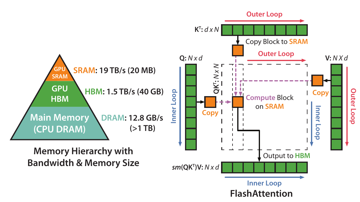
Figure 2. Memory hierarchy and attention tiling. Cropped from Dao et al., NeurIPS 2022 Figure 1, page 2; the performance panel is omitted. Hardware labels belong to the source example.5
That distinction matters: a more efficient attention kernel does not eliminate the KV cache, and an attention-only improvement is not the same as an equal improvement in total response time. For an explanation of attention and KV sharing, see Transformer attention.
Reuse context and schedule it carefully
Prefix caching saves an already computed prefix for reuse. It is useful when multiple requests share the same token prefix, such as a stable instruction plus a document. The Transformers guide provides a prefilled-cache example.2 Treat reuse as an execution contract: preserve the model, tokenizer, positions, attention policy and actual prefix token IDs. Similar wording is insufficient evidence that the cached numerical state remains valid.
Keeping a live conversation cache can save repeated prefill, but increases resident memory. A proposed application policy should decide when to retain, evict or reconstruct it. Scope shared state to the correct user and session; performance does not justify reusing another conversation’s context.
Chunked prefill divides prompt processing into smaller pieces while preserving the causal attention mask. It can create opportunities to interleave other work. SARATHI explains both the equivalence to full prefill and the costs of smaller chunks: lower arithmetic intensity and repeated reads of prior chunks’ KV state. Its reported scheduling gains are server results, not phone guarantees.1
For example, a proposed 2,048-token prompt processed in eight 256-token chunks offers seven boundaries at which an application might respond to cancellation or schedule another task. It does not permit a final answer to ignore the remaining prompt. Measure total prefill time and responsiveness together; a chunk size that improves one can worsen the other.
Speculative decoding trades extra work for fewer serial steps
A draft model proposes several tokens. The target model scores their prefixes together, keeps an accepted prefix, then produces a correction or one additional token. Leviathan et al.’s acceptance and correction rule preserves the target sampling distribution under the algorithm’s assumptions.6
Figure 3 shows why acceptance concerns a prefix, not independent votes on every proposed token. Once a proposal is rejected, later draft tokens conditioned on it cannot simply remain. The next iteration starts from the accepted and corrected continuation. Black, green, red and blue mark existing, accepted, rejected and corrected tokens respectively; the text here preserves that meaning without relying on color.7

Figure 3. Accepted prefix and corrected continuation. First three rows cropped from Leviathan, Kalman and Matias, ICML 2023 Figure 1, page 2. Original colors retained; CC BY 4.0.7
The mechanism is useful only if accepted tokens compensate for drafting, verification and discarded work. Their wall-time analysis assumes enough compute to verify candidates in parallel without increasing target-call time. Fewer target calls alone therefore do not establish faster execution on an edge device.6
For a proposed device experiment, measure a complete iteration rather than guessing from draft model size:
The numerator is seconds per iteration, including rollback and cache management; the denominator is average emitted tokens per iteration. Across variable iterations, use total time divided by total emitted tokens. Suppose these terms are 12 ms, 28 ms and 4 ms, and the mean emission is 2.2 tokens. The result is 20 ms/token. If the measured baseline is 18 ms/token, speculation is slower despite emitting multiple tokens per target call. These are illustrative numbers, not a published speedup. Include the extra model and state in peak memory and energy measurements.
Spend a budget appropriate to the task
Generating fewer tokens can reduce work, but truncating a needed explanation or reasoning trace changes the result. The s1 study demonstrates explicit control of thinking length; it also reports flattening gains and repetitive loops when forcing continued reasoning too often.8 A separate preprint challenges the interpretation of simple test-time scaling and reports inconsistent benefits from appending “Wait.” Treat that as scoped counterevidence, not a universal refutation of inference-time computation.9
A practical design is to evaluate several budgets on the actual task set, then choose the smallest that meets its quality target. A short classification, an extraction with a fixed schema and a difficult planning task need not share an output limit. Routing to a different model, skipping layers or shortening the context changes behavior and needs its own evaluation. See efficient models and agents and hybrid systems for those choices.
Streaming can make usable content available earlier, but does not itself remove model computation. Specify whether a token is merely generated, delivered to the application or visibly presented. A partial answer may still need validation before an application can act on it.
Match the intervention to the symptom
This table is a proposed diagnostic guide, synthesized from the mechanisms above. It is not a ranking of optimizations.
| Observed symptom | First question | Candidate intervention | Check the tradeoff |
|---|---|---|---|
| Long wait on first launch | Loading, compilation or prompt processing? | Retain a ready session; reuse valid compiled artifacts | Resident memory and app lifecycle |
| Long wait on a long prompt | Attention traffic, matrix work or input processing? | Reuse a valid prefix; suitable attention kernels | Cache validity and backend coverage |
| Slow answer after a quick start | Weight traffic, long-context attention or host overhead? | Better kernels, compression or less loop overhead | Quality, conversions and sustained throughput |
| Cancellation feels unresponsive | Where are the available scheduling boundaries? | Smaller execution chunks | Total latency and extra dispatch/cache reads |
| Speculation regresses | Are candidates accepted, and what does verification cost? | Adjust draft length or disable it for that workload | Peak memory and energy per task |
| Fast brief tests, slow long sessions | Does heat or resource contention change the path? | Reduce workload or revise concurrency | Sustained quality and task completion time |
Finish with evaluation and profiling: compare the completed task, including its quality, first response, full response, memory and energy. The fastest individual operator is valuable only when it improves the execution path the reader actually needs.
References
-
Amey Agrawal et al., SARATHI: Efficient LLM Inference by Piggybacking Decodes with Chunked Prefills, 2023, v1. Sections 2.2, 3.1 and 4.2; server-GPU study and chunking overheads. ↩ ↩2 ↩3 ↩4
-
Hugging Face, Cache strategies, Transformers main documentation inspected October 12, 2026. Fixed-size cache, offloading, quantized cache and prefill a cache sections; mutable documentation, not a claim of compatibility with every model. ↩ ↩2 ↩3
-
Joshua Ainslie et al., GQA: Training Generalized Multi-Query Transformer Models from Multi-Head Checkpoints, EMNLP 2023, v3. Section 2.2 and Figure 2 define shared KV heads. ↩ ↩2
-
Tri Dao et al., FlashAttention: Fast and Memory-Efficient Exact Attention with IO-Awareness, NeurIPS 2022, v2. Sections 2 and 3.1: tiled exact attention and memory traffic. ↩
-
Tri Dao et al., FlashAttention: Fast and Memory-Efficient Exact Attention with IO-Awareness, NeurIPS 2022 conference edition. Figure 1, page 2, memory-hierarchy and tiling panels; reproduced as a cropped excerpt for mechanism review. The runtime plot is omitted. ↩ ↩2
-
Yaniv Leviathan, Matan Kalman and Yossi Matias, Fast Inference from Transformers via Speculative Decoding, ICML 2023, v2. Algorithm 1 and Sections 3.3–3.5: sampling correction, hardware assumptions and extra arithmetic. ↩ ↩2
-
Yaniv Leviathan, Matan Kalman and Yossi Matias, Fast Inference from Transformers via Speculative Decoding, ICML 2023, PMLR 202:19274–19286. Figure 1, page 2, first three iterations only; published version distributed under the PMLR publication agreement, CC BY 4.0. ↩ ↩2
-
Niklas Muennighoff et al., s1: Simple test-time scaling, 2025, v1. Sections 3 and 4.2: budget forcing and limitations of continued reasoning. ↩
-
Guojun Wu, It’s Not That Simple. An Analysis of Simple Test-Time Scaling, 2025, v1 preprint. Abstract and Sections 3–4; a separate analysis of the simple scaling intervention. ↩