An efficient architecture spends the device’s limited memory and computation on the distinctions the task needs. A smaller weight file is only one part of that decision. The model also creates intermediate tensors, retains conversation state and moves data through a particular processor. Two models with similar parameter counts can therefore have very different deployment costs.12
This page connects architectural choices to those costs. Start with Edge AI foundations for the device budget and Transformer foundations for attention and feedforward blocks. The examples below are source inspection and calculations, not measurements on a phone. Sources and the released configuration were checked October 12, 2026.
Separate three kinds of size
Stored weights describe learned information shared across requests. Working activations are temporary tensors created while processing an input. Retained state survives between generation steps, such as attention’s keys and values. Compressing one does not automatically compress the others.34
For a dense decoder, a useful first approximation is a ledger of matrix sizes. Assume model width D, L independently parameterized layers, vocabulary V, gated feedforward width m, Hkv key/value heads and head width dh. Query width equals D. Input and output embeddings are tied; biases and small normalization vectors are omitted:
The four attention projections contribute two D by D matrices for queries and output, plus two D by Hkv·dh matrices for keys and values. A gated FFN contributes three D by m matrices. This is a Latent Light size derivation from the projection contracts, not a universal parameter formula: untied embeddings, expert banks, different head widths and shared layers change it.35
For decoding with full attention, the unreplicated KV payload is:
B is the number of simultaneous sequences, T their retained token count and sKV bytes per key or value element. The factor two counts K and V. This excludes allocator padding, cache metadata, temporary attention buffers and any physical duplication. A backend can allocate more than the logical payload.3
That distinction sets up the design questions: should we store fewer unique weights, keep fewer features per past token, or retain a compressed summary of the past?
Small decoders: allocate capacity deliberately
At sub-billion scale, vocabulary matrices can consume a substantial part of the budget. Tying the output projection to the input embedding reuses one matrix; reducing the vocabulary changes both storage and tokenization. The latter must be tested on the intended languages and inputs because a lower vocabulary count is not itself a lower sequence-processing cost.15
MobileLLM tested deep, narrow networks against wider, shallower networks at roughly 125M and 350M parameters. The deeper variants generally did better on the tested language tasks. Its immediate layer sharing applies the same block twice in succession, seeking additional transformations without adding another set of weights. These are results within that study, not a rule that maximizing depth always improves a device model.1
Reusing a block saves unique parameters but repeats computation. It may also improve weight locality when the same block remains in a fast cache. Whether that happens depends on the block’s size, backend scheduling and memory hierarchy. More layers still mean more dependent operations; parameter savings do not prove latency savings.1
- Load weights AOne learned transformation
- Apply block AProduce the next hidden state
- Load and apply BA second weight set and computation
Unique storage includes A and B. Each application processes a different hidden state.
- Load weights AOne weight set
- Apply block AFirst transformation
- Apply A againSecond transformation using the updated hidden state
Unique storage includes only A; the second computation remains. Cache residency and speed are implementation questions.
Figure 1. Weight reuse changes storage independently of execution depth. Original explanatory synthesis of MobileLLM’s immediate sharing mechanism.1
The shared path in Figure 1 is not equivalent to deleting a layer. It applies the transformation again to a new input. It also does not imply that the two applications can share their attention histories: those histories arise from different hidden states.
A worked footprint: the cache can exceed the weights
The released SmolLM2-135M base configuration makes a useful concrete ledger. It specifies L = 30, D = 576, m = 1,536, V = 49,152, nine query heads, three KV heads and tied embeddings. With ordinary equal-width query heads, dh = 576 / 9 = 64. Its configured context ceiling is 8,192; this is a configuration value, not evidence of equal quality at every length.5
Substituting into Equation (1) gives:
This omits normalization weights. If every counted parameter could be packed into exactly four bits, its payload would be 67.24 MB, or 64.13 MiB. This is an idealized calculation, not the size of an inspected quantized artifact: scales, zero points, padding and higher precision tensors add storage.
At one sequence, 4,096 retained tokens and two bytes per KV element, Equation (2) gives 94,371,840 bytes = 90 MiB. At 8,192 tokens it gives 180 MiB. The logical cache alone can exceed the ideal four-bit weight payload, despite the model having only about 135M parameters.
Keeping the layer count and head width fixed, replacing its three KV heads with nine would triple that cache to 270 MiB at 4,096 tokens; using one would reduce it to 30 MiB. These are hypothetical dimension changes, not interchangeable checkpoints or quality predictions.
Attention shares heads or limits history
Multi-head attention gives each query head its own K and V head. Multi-query attention (MQA) shares one pair across all query heads. Grouped-query attention (GQA) lies between them: each group of query heads shares a pair. Queries remain distinct. This reduces KV projection width and retained cache while preserving multiple query patterns.63
The GQA paper converts multi-head checkpoints by pooling KV projections within groups, then performs additional pretraining. Merely changing a configuration is not the demonstrated conversion procedure. Its quality and speed comparisons use the studied T5 models and hardware; they do not establish the result for every mobile decoder.3
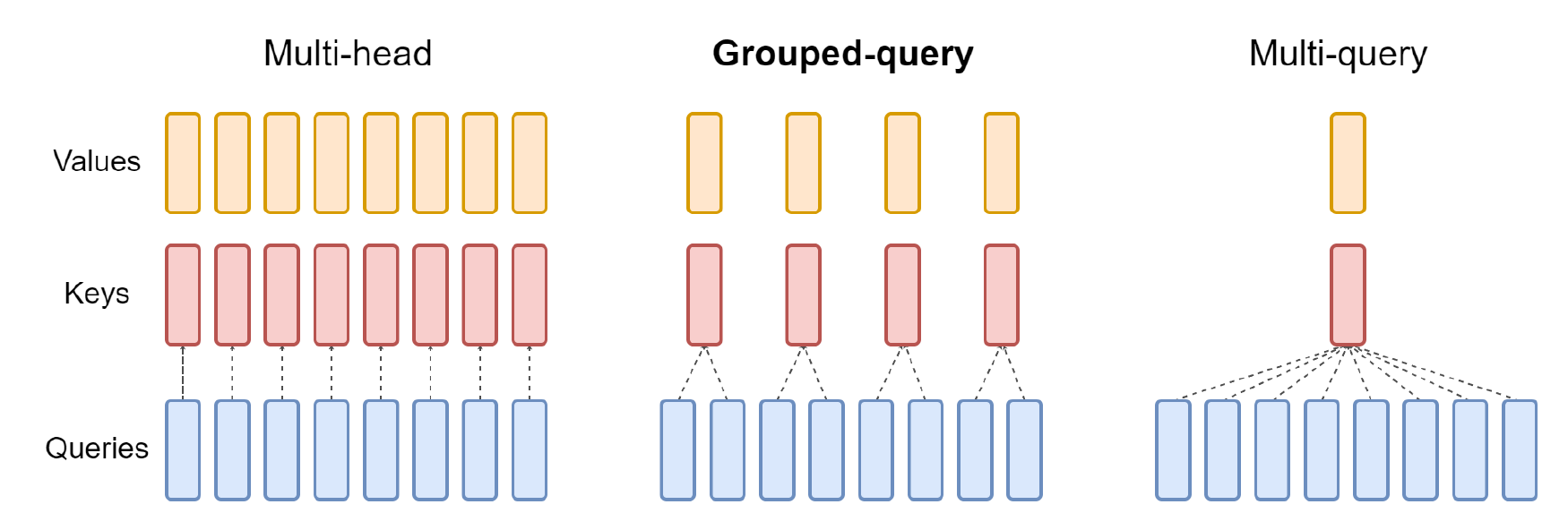
Figure 2. Queries stay distinct while keys and values are shared. Reproduced from Ainslie et al., GQA, EMNLP 2023, Figure 2; surrounding prose removed, original labels retained. © 2023 ACL, CC BY 4.0.7
Read the dashed connections in Figure 2: they show which queries read a common key head. The value heads above follow the same grouping. For the depicted eight queries, logical KV payloads scale as 8:4:1, with layer count, token count, head width and precision fixed. This is a shape ratio, not an 8:4:1 latency or quality comparison. The published figure’s eight heads are illustrative; the earlier SmolLM2 example has nine queries and three KV heads.7
Limiting attention to a rolling window changes a different dimension: T becomes at most the window length for those layers, if the runtime actually evicts old state. Alternating local and global layers only bounds the local layers. Gemma 2 is a worked example of that distinction; full-history layers still grow with context.8
| Design lever | Logical saving | What must be checked |
|---|---|---|
| Tied embeddings | One fewer vocabulary matrix | Checkpoint semantics and output head |
| GQA or MQA | Fewer KV features per past token | Quality after training, physical cache layout |
| Sliding window | Fewer retained positions in local layers | Old-state eviction and long-range task failures |
| Layer sharing | Fewer unique block weights | Repeated operations, separate state, locality |
| Recurrent or hybrid blocks | A summary state, possibly a bounded attention cache | Exact retrieval and supported kernels |
This table is a synthesis of the mechanisms above and below. The savings concern different objects and should not be added as independent speed multipliers.13842
Recurrence compresses the past
A recurrent model updates a fixed-size state rather than storing an addressable vector for every past token. Mamba makes parts of its state update input dependent, so it can select information to retain or forget. Its autoregressive state does not grow with context length for a fixed architecture and batch. That does not make every implementation fast: the paper’s hardware-aware scan is part of its contribution.4
The tradeoff is information access. Attention can revisit an earlier retained token; a recurrent block must recover what its state preserved. Griffin combines gated recurrence with local attention, retaining a compressed long-term route and a direct recent-token route. Its copying and retrieval experiments help reveal why those routes are complementary. They do not prove that every fact in a long prompt remains recoverable.2
This is a useful candidate for streaming tasks, but exact identifiers, quotations and rare facts deserve direct tests. A constant memory curve can coexist with a task failure curve that worsens as distractors or distances grow. Continue with Mamba for the selective update and efficient inference for the execution consequences.
Vision backbones spend spatial computation differently
For images, a compact architecture often separates spatial filtering from channel mixing. A depthwise convolution filters each channel independently; a pointwise convolution mixes channels. MobileNetV2 expands a narrow representation, applies depthwise filtering and projects back to a narrow linear bottleneck. Its residual path connects narrow representations, while nonlinear processing happens in the expanded space.9
This illustrates a broader principle: count the intermediate tensors as well as the stored weights. The paper describes an execution strategy that avoids fully materializing large intermediates. A generic implementation that does materialize them may have a different memory profile. For multimodal systems, the vision encoder, image resolution and number of features sent to the language model belong in the same budget; see multimodal Edge AI.9
Sparse experts are not small stored models
Mixture of experts selects a subset of FFN experts for each token. That limits active computation, while the other experts remain learned parts of the model. Mixtral’s paper explicitly distinguishes about 47B total from 13B active parameters and notes that serving memory follows total storage. Those rounded figures describe that large model; it is a mechanism example, not a phone recommendation.10
For an edge device, ask where every expert resides and how selected experts arrive. Offloading may trade resident memory for storage traffic and latency. Routing overhead, small per-expert batches and kernel support further affect execution. A dense small model can therefore be the more practical option even when a sparse model advertises a similar active count. Read Mixtral for routing and runtimes and compilers for backend constraints.10
The practical choice follows the workload: first set the task, maximum context, concurrency and input resolution; then compare actual weight, state and activation budgets. Training capable small models explains how to concentrate capability within that budget, quantization and compression changes its numerical representation, and evaluation and profiling establishes whether the complete system meets the target.
References
-
Zechun Liu et al. MobileLLM: Optimizing Sub-billion Parameter Language Models for On-Device Use Cases, ICML 2024, Sections 2.2–2.3 and 3.6. ↩ ↩2 ↩3 ↩4 ↩5 ↩6
-
Soham De et al. Griffin: Mixing Gated Linear Recurrences with Local Attention for Efficient Language Models, 2024, architecture, Section 6.2 and Appendix E. ↩ ↩2 ↩3
-
Joshua Ainslie et al. GQA: Training Generalized Multi-Query Transformer Models from Multi-Head Checkpoints, EMNLP 2023, Sections 2–3. ↩ ↩2 ↩3 ↩4 ↩5 ↩6
-
Albert Gu and Tri Dao. Mamba: Linear-Time Sequence Modeling with Selective State Spaces, 2024 edition, Sections 3.1–3.3 and 5. ↩ ↩2 ↩3
-
Hugging Face Smol Models Research. SmolLM2-135M configuration, released base artifact, dimensions and tied embeddings. Inspected October 12, 2026; no weights executed. ↩ ↩2 ↩3
-
Noam Shazeer. Fast Transformer Decoding: One Write-Head is All You Need, 2019, multi-query attention. ↩
-
Joshua Ainslie, James Lee-Thorp, Michiel de Jong, Yury Zemlyanskiy, Federico Lebrón and Sumit Sanghai. GQA: Training Generalized Multi-Query Transformer Models from Multi-Head Checkpoints, EMNLP 2023, Figure 2, printed page 4896. Figure covered by the ACL Anthology CC BY 4.0 policy; extraction and attribution record. ↩ ↩2
-
Gemma Team. Gemma 2: Improving Open Language Models at a Practical Size, 2024, Section 2 and Table 1. ↩ ↩2
-
Mark Sandler et al. MobileNetV2: Inverted Residuals and Linear Bottlenecks, CVPR 2018, v4, Sections 3 and 5. ↩ ↩2
-
Albert Q. Jiang et al. Mixtral of Experts, 2024, Sections 2.1 and 3, “Size and Efficiency.” ↩ ↩2