Quantization replaces a dense set of numerical values with a smaller set of representable levels. The aim is to keep the task’s useful behavior while reducing storage, memory traffic or arithmetic cost. Those are three different benefits: a smaller model file can still run through expensive conversions or unsupported operations.12
The central question is what is quantized, and how does the device compute with it? A W4A16 model uses four-bit weights and sixteen-bit activations. It says nothing by itself about the KV cache, accumulators, normalization or final output head. Start with efficient model architectures for the memory ledger and Edge AI foundations for device constraints.3
This is a mechanism study based on papers and official documentation inspected October 12, 2026. The numerical examples are calculations; no checkpoint conversion, training run or device benchmark was executed.
A quantizer is a numerical contract
An affine integer quantizer represents a real value x through integer q, positive scale s and integer zero point z:
The reconstructed value is x̂. Rounding loses detail; clipping loses range. The zero point makes real zero exactly representable, which matters for operations such as padded convolutions. Scales may belong to a whole tensor, a channel, a token or a group of weights. Different granularities create different accuracy, metadata and kernel requirements.14
Consider an illustrative symmetric four-bit quantizer using integers from −7 to 7, z = 0 and s = 0.2. It covers −1.4 to 1.4:
| Original x | Stored q | Reconstructed x̂ | Error x̂ − x |
|---|---|---|---|
| −0.72 | −4 | −0.80 | −0.08 |
| 0.13 | 1 | 0.20 | 0.07 |
| 0.93 | 5 | 1.00 | 0.07 |
This is a Latent Light calculation from Equation (1), not a published model measurement. Without clipping, round-to-nearest error is at most half a step. If an outlier of magnitude eight forces the same group’s scale to 8 / 7, the step becomes about 1.143. Values near zero now have much coarser representation.
Smaller groups can isolate an outlier, but require more scales. Clipping it keeps a finer step for ordinary values but damages that outlier. Whether that is acceptable depends on its effect on the layer output and task, not simply on how rare it is.4
Four bits is not exactly four bits of storage
For a group of g weights, nominal weight precision b and m metadata bits per group, the ideal packed storage is:
For 128 four-bit weights plus one sixteen-bit scale, the group occupies 64 + 2 = 66 bytes, or 4.125 bits per weight. The ideal ratio relative to FP16 is 16 / 4.125 ≈ 3.88, before padding, zero points, headers or tensors left in higher precision. This derivation assumes that all groups use this exact representation. A format name alone does not establish it.
Keep three ledgers: file bytes, peak resident memory and runtime traffic. Unpacking the whole model into FP16 at load time could erase the resident saving; fused dequantization can retain packed weights while reconstructing values near the computation.3
PTQ and QAT solve different preparation problems
Post-training quantization (PTQ) starts with a trained model and chooses a representation, often using calibration inputs. These inputs reveal ranges, activation patterns or how errors affect layer outputs. “No retraining” does not mean “no data” or “no preparation computation.”53
Quantization-aware training (QAT) updates model weights while simulating the target rounding and clipping in its forward pass. Fake quantization can leave tensors in floating point while reproducing quantize/dequantize numerics. A straight-through gradient approximation commonly allows optimization through rounding. The resulting model still needs conversion to a real deployment representation.16
- Trained model + samplesRun calibration inputs through the existing model
- Choose scales and weightsObserve ranges or reconstruct layer outputs
- Pack for the backendStore low-bit values and required metadata
Model training is not repeated, but preparation may optimize rounding or compensate errors.
- Insert fake quantizersSimulate the intended rounding and clipping
- Update floating weightsTrain while exposing quantization error
- Convert and packReplace simulation with the deployment format
The training graph must match the eventual precision, grouping and operation boundaries. Fake quantization alone is not an inference kernel.
Figure 1. Two preparation routes, one requirement: match the target computation. Original synthesis informed by GPTQ, Jacob et al. and PyTorch’s QAT explanation.516
As Figure 1 shows, QAT adds an opportunity to adapt weights to error; it also adds training cost and data requirements. PTQ is a useful first candidate. If it misses the quality target, investigate calibration, sensitive layers and representation before assuming that every operation needs retraining.
GPTQ, AWQ and SmoothQuant: three error-control ideas
| Method | Main target in the cited work | How it controls error | Deployment implication |
|---|---|---|---|
| GPTQ | Low-bit weights | Reconstruct layer outputs using calibration inputs; compensate remaining weights as columns are quantized | Requires a matching packed representation and kernels |
| AWQ | Low-bit weights | Use activation statistics to identify salient channels and search an equivalent channel scaling | Protects channels without requiring a permanent mixed-precision exception for each salient weight |
| SmoothQuant | Eight-bit weights and activations | Move activation magnitude variation into weights with a compensating rescaling | Designed around W8A8 matrix operations |
This comparison is a mechanism synthesis, not a ranking of current implementations.534
GPTQ approximates a layer reconstruction problem: choose quantized weights whose outputs resemble the original outputs on calibration inputs. Its second-order information comes from those layer inputs. Quantizing one column changes the remaining floating weights to compensate; block updates and a Cholesky formulation make the procedure practical. It is not an end-to-end task-loss optimizer, and its original results do not quantize activations.5
AWQ asks which weight channels matter most under the input activations. Large activation magnitudes can amplify error in the corresponding channels. Rather than leave a small collection of salient weights in FP16, it searches scales that protect those channels while preserving a uniform low-bit weight format. The paper reports calibration-generalization benefits; that is evidence for its tested distributions, not immunity to arbitrary distribution shift.3
SmoothQuant addresses activation outliers. With row-vector activations X, weight matrix W and positive diagonal scaling S, the floating-point linear operation can be rewritten:
S scales input channels; its inverse counteracts the scale on activations. This is algebraically equivalent before rounding. After quantization, the two sides have different errors. SmoothQuant chooses a balance that makes activation ranges easier to quantize while keeping weights manageable. The method’s identity is W8A8 preparation, not a generic synonym for four-bit weights.4
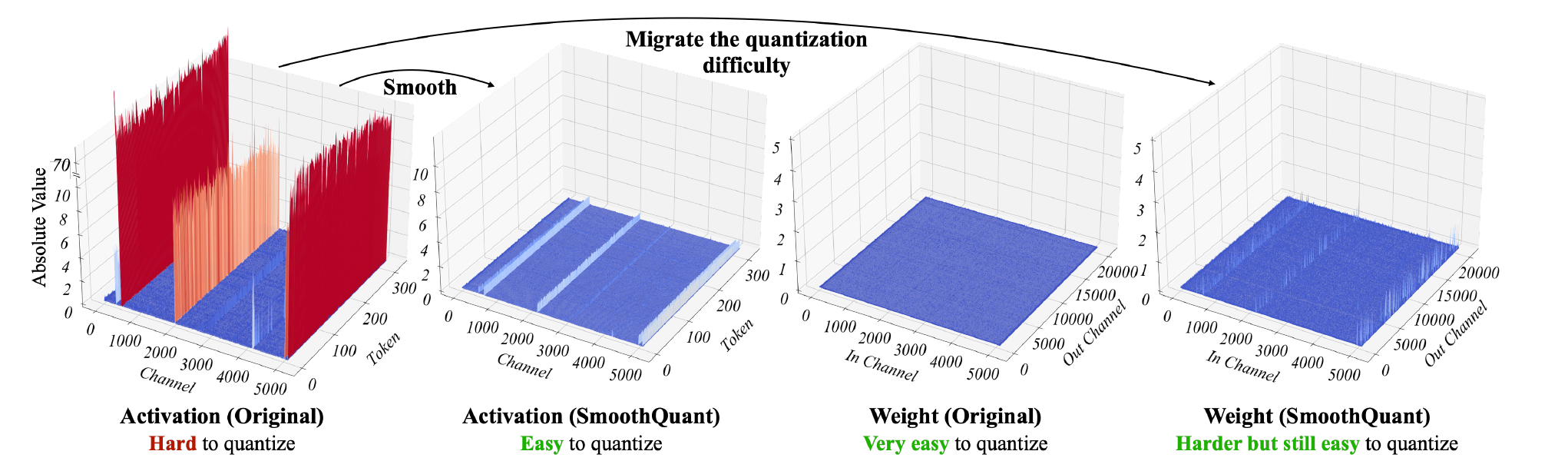
Figure 2. Rescaling moves the difficult range between activations and weights. Reproduced from Xiao et al., SmoothQuant v5, Figure 4, PDF page 4; surrounding prose removed. © 2023 the authors, CC BY 4.0.7
Figure 2 is an author-reported observation for one OPT-13B linear layer, not a statement that every small model has the same outliers. The first panel shows large values recurring in particular input channels across tokens. After scaling, activation magnitude is easier to represent, while the weight range becomes less uniform. Notice the differing vertical scales: visual height cannot be compared as if every panel used one range. The figure shows magnitude redistribution, not model accuracy, device latency or memory consumption.7
All three use information about input behavior. Their methods and comparisons do not justify taking a speedup reported on one GPU, batch and sequence length as a prediction for a phone.
Calibration must resemble the difficult inputs
A practical calibration set should exercise the actual preprocessing and input distribution: chat templates, languages, code or structured fields, prompt lengths, images or audio where supported, and rare but important cases. Keep calibration separate from the final test set. This is a proposed evaluation design informed by data-dependent quantization, not a universally optimal sample count.53
Static activation quantization determines ranges in advance. Dynamic quantization computes ranges at runtime, adding work while adapting to each input. ONNX Runtime documents both approaches and several calibration methods, including MinMax, Entropy and Percentile. Their suitability depends on the model and execution provider.2
Compare the original and converted models on the same held-out tasks. Perplexity or layer reconstruction error is informative but does not alone establish exact extraction, reasoning, tool arguments or safety behavior. Inspect failures by slice; a modest average change can hide a large regression on a rare input class.
The KV cache is a separate compression target
Weight quantization leaves the per-request cache unchanged unless a separate cache scheme is selected. KIVI studies low-bit KV storage and finds different useful axes for keys and values in the tested models: keys per channel and values per token. It retains a recent full-precision residual buffer while quantizing grouped older entries.8
That residual is substantive. In the paper, quantizing every token in a simulated two-bit cache hurts difficult generation tasks more than the actual KIVI scheme. Its “two-bit cache” therefore does not mean every retained byte uses two bits. Scales, residual state and mixed-precision attention all belong in a memory calculation.8
Cache quality depends on length and content. Test distant exact retrieval, repeated distractors and generation length, not just a short prompt. Reducing cache precision and reducing its attention window are separate interventions: one changes numerical fidelity, the other changes which history is visible.
Pruning needs an executable sparsity pattern
Pruning sets selected weights to zero or removes structures such as channels, heads or blocks. Unstructured pruning can preserve matrix shapes; a dense kernel still processes those shapes. Structured pruning can shrink them but removes larger units of capacity. SparseGPT demonstrates efficient one-shot pruning with layer reconstruction and discusses both unstructured and hardware-compatible patterns; its quality results do not automatically establish a speedup on every device.9
For a concrete backend constraint, TensorRT’s 10.x documentation specifies a 2:4 pattern: at least two zeros in each group of four along the required reduction dimension. Eligible weights, enabled sparsity and supported hardware are still insufficient to guarantee that the builder chooses a sparse tactic. It can select a dense one when that is faster. Check the resulting engine and measure the complete workload.10
Pruning and quantization can be combined, but their errors need joint evaluation. Distillation can recover or transfer useful behavior during compression; training capable small models covers that objective.
The format, graph and kernel must agree
Record the weight and activation dtypes, scale axes, group size, symmetric or asymmetric scheme, zero-point representation, packed layout, accumulator precision and cache dtype. A quantization algorithm is not a portable file format. Backend conversion is part of the model’s numerical contract.
ONNX Runtime illustrates the specificity: its documented four-bit path is blockwise weight-only quantization for selected operations with constant weights. MatMul can become MatMulNBits or a DequantizeLinear/MatMul pair; Int4 and UInt4 require ONNX opset 21. This does not promise low-bit execution for an arbitrary graph or execution provider.2
The same documentation warns that quantization can be slower when hardware lacks efficient instructions or conversions dominate. Follow runtimes and compilers to inspect delegation and fallback, efficient inference to understand memory traffic, and evaluation and profiling to measure time to first token, sustained generation, memory and energy under the actual workload.2
References
-
Benoit Jacob et al. Quantization and Training of Neural Networks for Efficient Integer-Arithmetic-Only Inference, CVPR 2018, Sections 2–3. ↩ ↩2 ↩3 ↩4
-
Microsoft. Quantize ONNX models, representation formats, calibration, Int4/UInt4 and performance FAQ. Inspected October 12, 2026. ↩ ↩2 ↩3 ↩4
-
Ji Lin et al. AWQ: Activation-aware Weight Quantization for On-Device LLM Compression and Acceleration, MLSys 2024, Sections 3–5. ↩ ↩2 ↩3 ↩4 ↩5 ↩6
-
Guangxuan Xiao et al. SmoothQuant: Accurate and Efficient Post-Training Quantization for Large Language Models, ICML 2023, Sections 2–4. ↩ ↩2 ↩3 ↩4
-
Elias Frantar et al. GPTQ: Accurate Post-Training Quantization for Generative Pre-trained Transformers, ICLR 2023, v2, Sections 3–4 and the original activation-quantization boundary. ↩ ↩2 ↩3 ↩4 ↩5
-
PyTorch. Quantization-Aware Training for Large Language Models with PyTorch, July 2024, fake quantization, straight-through gradients and conversion. This is the dated method explanation, not a claim about the latest torchao API. ↩ ↩2
-
Guangxuan Xiao, Ji Lin, Mickael Seznec, Hao Wu, Julien Demouth and Song Han. SmoothQuant: Accurate and Efficient Post-Training Quantization for Large Language Models, ICML 2023, v5 dated June 5, 2023, Figure 4 and Sections 3–4. The versioned report identifies CC BY 4.0; extraction and attribution record. ↩ ↩2
-
Zirui Liu et al. KIVI: A Tuning-Free Asymmetric 2bit Quantization for KV Cache, ICML 2024, Sections 3 and 4.2.1. ↩ ↩2
-
Elias Frantar and Dan Alistarh. SparseGPT: Massive Language Models Can Be Accurately Pruned in One-Shot, ICML 2023, Sections 2–4. ↩
-
NVIDIA. TensorRT I/O Formats: Sparsity, 10.x documentation, required weight pattern and tactic selection. Inspected October 12, 2026. ↩