A camera produces pixels. A useful vision system has to turn those pixels into answers: what is here, where is it, and can I respond in time? A robot needs to locate the object it will approach. An inspection station needs to find a defect while the part is still in view. A visual assistant needs a useful answer from the current scene, rather than an accurate description of a frame that has already passed.
YOLO made a powerful proposal: predict object locations and categories together with one neural network looking at the whole image. Its original 2015 paper called this You Only Look Once. What followed is a broad research ecosystem: new ways to represent boxes, share features, assign training targets, remove duplicate predictions and fit real hardware.1
The central idea has endured; the implementation has changed substantially. Modern YOLO is a branching family of detectors and software projects. A larger version number does not establish authorship, direct ancestry or superior performance for a particular application. Figure 2 maps the main branches and the ideas that connect this tutorial.
The animation in Figure 1 previews the detection idea.
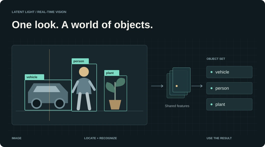
Figure 1. From pixels to objects. An original schematic animation of joint localization and recognition; the scan, timing, objects and outputs are illustrative. The family map in Figure 2 connects this idea to the rest of the tutorial.
One idea. A branching family.
Predict object locations and categories together. A decade of research changes how features, training and deployment make that possible.
YOLO26Released
YOLO27Preview
v14 paperWithdrawn
A curated family map, not a literal code ancestry tree or an accuracy ranking. Arrows within the original and Ultralytics rows show their release sequences; dots group related work without asserting direct inheritance. Dates are first paper years except software releases; YOLOv6 also shows its 2023 revision. Status checked November 8, 2026.
Figure 2. The YOLO landscape at a glance: origins, parallel research directions, the Ultralytics software family and open-vocabulary extensions. This independent synthesis groups contributions by their authors and purpose. It does not draw unsupported inheritance edges. Current release status comes from the official artifacts and paper records.123456789101112131415
Reading routes
- Learn the ideas: start with the original detector, then follow the modern pipeline and training and assignment.
- Understand the family: use the model map and the development story.
- Build with it: read the current YOLO26 contract, measurement and the deployment workflow.
Evidence checked November 8, 2026. YOLO26 is the latest released Ultralytics family; YOLO27 is a preview without public model artifacts. The arXiv paper named YOLOv14 was withdrawn by its authors. These are separate statuses, not three interchangeable candidates.161213
What detection is trying to solve
Image classification gives an image-level label. Object detection returns a set of objects, usually represented by a class, a bounding box and a score. Instance segmentation adds a mask for each object; pose estimation adds keypoints. Tracking associates detections across time. These tasks can share features or a software API, but they have different outputs and evaluation rules.
For axis-aligned detection, a box might be stored as its center and dimensions
(cx, cy, width, height) or as corners (x1, y1, x2, y2). Coordinates might be
normalized, measured in the resized model input or mapped back into the original
image. An apparently plausible box can still be wrong if those conventions are
mixed.
Before YOLO, influential detection pipelines generated candidate regions and classified them through a sequence of operations. The original paper’s target was that fragmented design: share image computation, learn localization and recognition together, and make detection fast enough to participate in a live system. It also reported a trade-off: fewer background false positives than some contemporary methods, but substantial localization errors and difficulty with groups of small objects. Those were findings about the original detector, not permanent properties of every model subsequently called YOLO.1
“One look” means a single network evaluation for the image. It does not mean one predicted box, one feature resolution, one operation or an absence of post-processing. The original YOLO used non-maximum suppression.
The original idea
A grid assigns responsibility
Original YOLO divides the image into an S × S grid. The cell containing an object’s center is responsible for that object. Each cell predicts B boxes, with five values per box, and one vector of C conditional class probabilities. The class vector is shared by the cell’s boxes. Figure 3 makes that ownership rule concrete.1
The object’s center chooses the cell.
A 7 × 7 grid assigns responsibility. Each cell predicts two boxes and one shared vector of 20 class probabilities in the original VOC setup.
Per cell
2 × 5+20=30
Two boxes: x, y, w, h, confidence
One shared class vector
The highlighted cell contains the center of the illustrated object. The object can extend beyond the cell: the grid assigns responsibility, not box boundaries. For each cell, 2 × 5 box values plus 20 class values give 30 numbers; 7 × 7 × 30 = 1,470 raw outputs and 98 candidate boxes.
Original YOLO example: S=7, B=2, C=20. The scene is an independent schematic, not a detector output. Modern YOLO models use different spatial scales, score definitions and head contracts.
Figure 3. The grid assigns responsibility; it does not confine the predicted box. The original PASCAL VOC example produces a 7 × 7 × 30 tensor. The highlighted cell, object and box are explanatory geometry, not a recorded prediction.1
For each original box, x and y locate the center relative to its cell;
w and h describe dimensions relative to the whole image. The confidence
term was defined as the probability of an object multiplied by predicted
intersection over union. Multiplying this by the cell’s conditional class
probability yields the original class-specific score:1
Here, b is the predicted box and the IoU term concerns its overlap with the
matched ground-truth box. This is the original training interpretation of the
score; ground truth is not available to compute IoU at inference. The network
learns to predict the confidence term.
Do not copy that formula onto every YOLO head. Some later implementations have explicit objectness channels; others predict class scores without a separate objectness output. The inspected modern Ultralytics detection head applies sigmoid to class logits and decodes its box branch separately.17
A unified model, with real constraints
The original detection network had 24 convolutional layers followed by two fully connected layers. Its fixed grid and shared class prediction constrained nearby objects. For training, one of a cell’s box predictors became responsible for an object according to current IoU. The loss combined coordinate, confidence and classification terms, with special weighting for background and localization. The paper itself noted that squared error did not align perfectly with average precision.1
The lesson is broader than the historical architecture: detection requires a contract between representation, assignment, loss and inference. Changing one can alter the behavior of the others. Later YOLO research changes all four, rather than merely adding more layers to the original network.
Inside a modern YOLO detector
A useful starting model is backbone → neck → head. It is a conceptual organization, not a promise that every architecture has identical boundaries. Some modern designs exchange features across those boundaries or incorporate attention within otherwise convolutional networks.18910
- Backbone: extract increasingly abstract features, commonly at decreasing spatial resolution.
- Neck: combine features across resolutions so fine spatial information and broader semantic context can meet.
- Head: turn those features into box parameters, class scores and, for other tasks, masks, keypoints or angles.
Figure 4 follows this shared computation into three prediction scales.
One image. Shared features. Several spatial scales.
A backbone extracts features; a neck exchanges information across resolutions; a head predicts boxes and class scores at each output location.
640 × 640 example8,400 prediction locations
For a 640 × 640 input and output strides 8, 16 and 32, the feature grids are 80 × 80, 40 × 40 and 20 × 20. One prediction point per location gives 6,400 + 1,600 + 400 = 8,400 locations. All levels can detect objects; the labels describe spatial sampling, not hard object-size restrictions.
This matches a common three-level anchor-free setup, including the inspected YOLO26 YAML. It is not universal: input aspect ratio, added pyramid levels, multiple box priors and the export path change the contract.
Figure 4. A common modern three-scale detector. Grid textures are symbolic; the numerical dimensions are calculated for a 640 × 640 input with strides 8, 16 and 32. The inspected YOLO26 configuration uses those output strides.17
Multi-scale features address a sampling problem
Repeated downsampling makes computation cheaper and expands context, but small objects occupy fewer feature locations. Combining a finer feature map with information from deeper layers helps the detector retain spatial detail. YOLOv3 made three-scale prediction a prominent part of the family’s design; later necks build increasingly elaborate routes for sharing information.18
A high-resolution head does not exclusively detect small objects, and a coarse head does not exclusively detect large ones. Target assignment and learned features determine which predictions become useful. Raising input resolution, adding a finer feature level or tiling an image can help a small-object problem, but each changes computation, memory use and the evaluation protocol.
Anchors, anchor points and anchor-free prediction
An anchor box is a reference width and height against which a detector predicts adjustments. YOLOv2 used clustering of training box dimensions to choose those priors. YOLOv3 continued this approach across several scales.1918
An anchor-free head avoids a predefined collection of box shapes at every location. It can predict a box from a feature-map point, for example through distances to the box’s four sides. It still needs a spatial reference and an assignment rule. Source code may call those reference points “anchors”; that name does not necessarily mean anchor-box priors are present.417
The distinction concerns box representation. It does not decide whether NMS is needed. YOLOX is an important anchor-free design, while YOLOv10 investigates NMS-free training through a separate assignment mechanism.48
Decoupled heads and distributional regression
Classification asks which category a region belongs to. Localization asks how precisely its boundaries should be placed. A decoupled head gives those objectives separate prediction branches after shared features. YOLOX made that design choice explicit and studied its effect on optimization.4
Another distinction is how a box side is represented. In a head using
Distribution Focal Loss (DFL), a side distance is represented by a distribution
over discrete bins and decoded by its expectation. This adds regression logits;
it is not simply an extra class confidence. For a head with R bins and C
classes, a common raw per-location contract is 4R + C logits. After decoding,
the box becomes four coordinates, so the decoded contract can be 4 + C.
YOLO26 sets reg_max=1 and removes the DFL distributional decoder.1117
For example, 80 classes and 16 regression bins give 144 raw values per location, not 144 decoded coordinates. The comparable direct-regression example has 84. This arithmetic describes a selected head design; it is not a universal formula for every YOLO model or export.
How training teaches a detector
The model can produce thousands of predictions from one image. Training must decide which of them should explain each annotated object, what the others should learn, and how localization and recognition errors should be weighted.
Assignment connects annotations to predictions
Label assignment chooses positive predictions for each ground-truth object. The assignment might depend on geometric constraints, predicted overlap, classification scores or a matching cost. It can change as the model learns. YOLOX’s SimOTA is one influential dynamic assignment approach. Later work uses task-aligned scores to encourage predictions that both recognize the class and localize the object.48
One-to-many assignment provides several positives for one object. That supplies rich supervision, but it also teaches multiple predictions around the same instance. One-to-one assignment selects one positive prediction per object. This supports a unique-output inference path, although training and convergence require care. The important distinction is the number of matched predictions, not whether the network is a CNN or a Transformer.820
Losses and recipes are part of the model
A contemporary detection objective commonly includes classification and localization losses, and sometimes a distributional box loss or auxiliary objectives. Assignment determines where those losses apply. Positive/background imbalance, classification quality and box overlap interact, so a different loss cannot be assessed independently of its targets and training recipe.
Augmentation, initialization, pretraining data, optimizer, resolution, training duration and model selection also matter. Mosaic combines image regions from several training examples; other augmentation choices alter color, scale or geometry. Strong augmentation can improve robustness, but a policy that helps one model size or domain may damage another. YOLOv4 and YOLOX are useful primary sources for the importance of the complete recipe.24
A reported gain attributed to a new architecture can therefore include changes in data and optimization. Read the ablations and training disclosure before calling it a pure architecture improvement.
NMS-free does not mean no post-processing
Non-maximum suppression (NMS) ranks candidate boxes and suppresses competing overlaps according to a chosen policy, often within each class. Its overlap threshold controls suppression, while the score threshold controls which predictions are considered. These are different decisions. Crowded scenes can make suppression difficult because two real nearby objects may overlap. Figure 5 contrasts suppression with one-to-one prediction.
Remove duplicates—or train a head to avoid them.
Anchor-free describes box parameterization. NMS-free describes duplicate handling. They answer different questions.
Dense head + NMS
Match several candidates during training; suppress overlapping detections at inference.
One-to-one head
Train toward unique assignment; select predictions without an IoU suppression pass.
In the dense-prediction path, several candidates overlap one object; NMS keeps the strongest candidate and suppresses competing overlaps according to a chosen policy. In the one-to-one path, assignment trains a head toward one selected prediction per annotated object; inference uses decoding and selection without IoU-based suppression.
Illustrative boxes and scores, not measurements. One-to-one training does not guarantee perfect uniqueness on every image. Thresholding, top-k selection and coordinate transforms can remain in an NMS-free pipeline.
Figure 5. Two ways to address duplicate predictions. The scores and geometry are illustrative. A one-to-one training rule encourages a unique prediction; it does not guarantee every real image will contain neither duplicates nor misses.817
YOLOv10 couples a one-to-many branch with a one-to-one branch during training, using consistent matching metrics. The dense branch supplies supervision; the one-to-one branch supplies the inference path without NMS. Its matching rule aligns the preferences of the two branches instead of treating them as unrelated objectives. The original head schematic in Figure 6 shows the two branches sharing their feature extractor.8
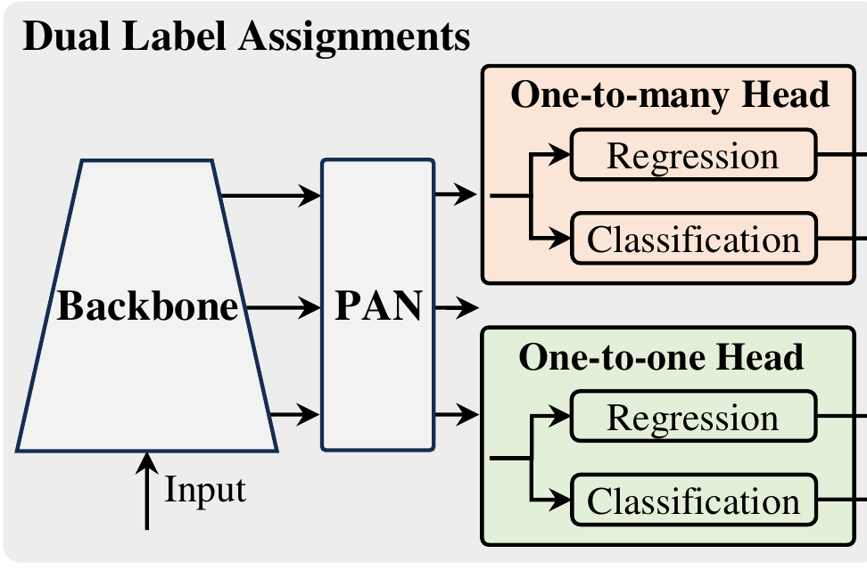
Figure 6. Original head-structure portion of YOLOv10 Figure 2(a), by Ao Wang and colleagues, arXiv v1, page 4. Cropped to omit the matching panels, embedded photograph and chart; right-edge outputs continue outside the crop. Reused under CC BY 4.0. The full figure explains consistent matching between these branches.8
NMS-free inference can still decode distances into boxes, apply a score
threshold, select a bounded number of predictions and undo input resizing and
padding. In the inspected Ultralytics implementation, a function named
non_max_suppression even contains an early path for E2E outputs that filters
predictions without running IoU-based NMS. Follow the executed branch, rather
than inferring behavior from a function’s name.17
Model map at a glance
This map separates who developed the model, when it first appeared and what idea is useful to study. Dates below are first paper dates unless marked as software releases. Later revisions can substantially change a family. “Released” means a documented public model/code release; it does not mean we ran every checkpoint or reproduced its results.
YOLO families and contributions
19 families| Model / first appearance | Author or project | What to learn from it | Evidence / status | Official implementation license |
|---|---|---|---|---|
| YOLO v1 · Jun 2015 | Redmon, Divvala, Girshick, Farhadi | Joint whole-image box/class regression; grid responsibility | Paper and original method | Public-domain dedication (Darknet) |
| YOLOv2 / YOLO9000 · Dec 2016 | Redmon, Farhadi | Learned box priors, multi-scale training; joint detection/classification | Paper | Public-domain dedication (Darknet) |
| YOLOv3 · Apr 2018 | Redmon, Farhadi | Darknet-53 and three-scale predictions | Technical report | Public-domain dedication (Darknet) |
| YOLOv4 · Apr 2020 | Bochkovskiy, Wang, Liao | CSP backbone, feature fusion and an effective training recipe | Paper / Darknet | Public-domain dedication (Darknet) |
| YOLOv5 · Jun 2020 software release | Ultralytics | PyTorch training/deployment workflow and scaled models | Original repository; distinguish v5u | AGPL-3.0; v7.0: GPL-3.0 |
| YOLOX · Jul 2021 | Ge et al., Megvii | Anchor-free decoupled head and SimOTA | Paper / author code | Apache-2.0 |
| YOLOv6 · Sep 2022; v3 report Jan 2023 | Meituan | Industrial efficiency; reparameterization, training auxiliaries | Original report / v3 report | GPL-3.0 |
| YOLOv7 · Jul 2022 | Wang, Bochkovskiy, Liao | E-ELAN, scaling and trainable bag-of-freebies | Paper / author code | GPL-3.0 |
| YOLOv8 · Jan 2023 software release | Ultralytics | Anchor-free split head and a multi-task software family | Official docs | AGPL-3.0 |
| YOLOv9 · Feb 2024 | Wang, Yeh, Liao | PGI training supervision and GELAN architecture | Paper / author code | GPL-3.0 |
| YOLOv10 · May 2024 | Wang et al., THU-MIG | Consistent dual assignment and efficiency-driven design | Paper / author code | AGPL-3.0 |
| YOLO11 · Sep 2024 software release | Ultralytics | Refined blocks and a practical multi-task implementation | Official docs | AGPL-3.0 |
| YOLOv12 · Feb 2025 | Tian, Ye, Doermann | Area attention and residual feature aggregation | Paper / author repo | AGPL-3.0 |
| YOLOv13 · Jun 2025 | Lei et al., iMoonLab collaborators | HyperACE and FullPAD feature exchange | Paper / author repo | AGPL-3.0 |
| YOLO26 · Jan 2026 software release; Jun 2026 report | Ultralytics | DFL-free regression, dual heads and coordinated training | Report / released code | AGPL-3.0 |
| YOLO-World · Jan 2024 | Cheng et al., Tencent / collaborators | Efficient text-conditioned open-vocabulary detection | Paper / author code | GPL-3.0 |
| YOLOE · Mar 2025 | Wang et al., THU-MIG | Text, visual and prompt-free detection / segmentation | Paper / author code | AGPL-3.0 |
| YOLOE-26 · described in Jun 2026 report | Ultralytics | YOLOE prompting on the YOLO26 detector family | Report §3.6 | AGPL-3.0 |
| YOLO27 · preview as checked Nov 2026 | Ultralytics | Planned small CNN / larger query-based designs | Preview only; no public model artifacts | Not released; model terms pending |
No matching families. Try another term or reset the search.
Scroll to compare. Focus view gives the table more room.
License scope (checked November 11, 2026): the column identifies the linked author/project implementation, not a blanket license for every checkpoint, dataset, dependency or third-party integration. Original Darknet uses its custom public-domain dedication. Current YOLOv5 is AGPL-3.0; its v7.0 release was GPL-3.0. Ultralytics also offers Enterprise licensing. Choose the terms attached to the exact artifact you use; paper-figure licenses are separate. YOLO27 has no released model artifact whose license can be listed.
A naming trap: the YOLOv14 arXiv record was withdrawn in version 4 on August 20, 2026. It belongs in a research-status note, rather than a released successor ranking. A similarly named repository is not evidence of a shared author or a valid benchmark.13
How the family developed
From grid regression to multi-scale detection
YOLOv2 improved the original detector through a collection of changes, including batch normalization, learned box dimension priors and multi-scale training. Replacing the fixed fully connected detection endpoint with a fully convolutional approach also made variable input sizes practical. The companion YOLO9000 work used a hierarchical label structure, WordTree, to combine classification and detection supervision. A larger category vocabulary did not mean dense detection annotations existed for every category.19
YOLOv3 introduced Darknet-53 and predictions from three feature scales, with upsampling and feature combination. Its class predictions used independent logistic classifiers rather than forcing every prediction into a single softmax category. That was useful for nonexclusive labels. Its report also illustrates why AP50 and stricter localization metrics can tell different stories.18
These models established several long-lived themes: share image features, predict densely, mix semantic context with spatial detail, and make box parameterization learnable. Their precise tensors and score definitions should still be read in the original edition, rather than reconstructed from the modern Ultralytics API.
Training and gradient design
YOLOv4 was developed by Alexey Bochkovskiy, Chien-Yao Wang and Hong-Yuan Mark Liao. It combined a CSPDarknet53 backbone with spatial pyramid pooling and path aggregation, alongside a broad training recipe. Its useful distinction is between changes that improve learning without adding inference work and changes that alter the inference architecture. The paper treats effective combinations and ablations as central research work.2
YOLOv7 developed this training-centered direction further: extended efficient layer aggregation (E-ELAN), model scaling, planned reparameterization and lead/auxiliary-head supervision. Reparameterization can use a richer training structure that is algebraically converted into a simpler inference structure. It is different from merely deleting useful layers after training.6
YOLOv9 separates two contributions. GELAN is the efficient feature aggregation architecture. Programmable Gradient Information (PGI) is a training supervision framework, with auxiliary paths intended to improve the learning signal. The report’s inference path uses the main branch. Describing PGI as an extra inference-time reasoning network would misunderstand its purpose.7
These papers share collaborators and research themes. That does not make every model a strict checkpoint-compatible successor or establish a direct code edge between every pair in the overview.
The Ultralytics software family
YOLOv5 developed as an Ultralytics PyTorch project, with accessible training, evaluation, exports and several model sizes. Its software workflow was a substantial part of its contribution. Use its repository and tagged releases as primary evidence, rather than inventing a definitive v5 paper to fill a timeline.3
The name now has an extra ambiguity: YOLOv5u uses an anchor-free,
objectness-free split head related to YOLOv8. Current documentation explicitly
distinguishes it from original ultralytics/yolov5 checkpoints and their loader
compatibility. A row labeled “v5” must identify which artifact is being
evaluated.21
YOLOv8, released January 10, 2023, made an anchor-free split head part of a multi-task software family. YOLO11, released September 27, 2024, refined feature extraction and the implementation; its released configuration includes C3k2 and C2PSA blocks. The presence of attention in such a model is one reason “YOLO means pure convolution” is an unreliable definition.222317
YOLO26 continues this software lineage with direct box regression, selectable NMS/NMS-free heads and a coordinated training recipe. Its public launch was January 14, 2026; the primary report followed on June 2. An announcement, a software release and a paper submission are different events.1611
Parallel paths to efficient detection
YOLOX is a Megvii research project, not a numbered Ultralytics release. Its anchor-free prediction, decoupled head and SimOTA assignment offer a particularly clear case study of interactions between representation and training. Anchor-free heads still produced dense candidates that needed an inference selection policy.4
YOLOv6, developed at Meituan, emphasizes industrial efficiency. Its v3.0 report adds a RepBi-PAN neck, anchor-aided training and a self-distillation strategy. Auxiliary anchor-based or heavier regression branches can strengthen training while being removed from the inference path. This is another example of why the training graph and deployed graph should be examined separately.5
YOLOv10, from THU-MIG, combines consistent dual assignments with a broader architecture study. Lightweight classification heads, spatial/channel-decoupled downsampling and rank-guided block allocation address computation; large-kernel convolutions and partial self-attention address representation. NMS removal is one contribution within that coordinated design.8
A CNN can therefore be NMS-free, and an efficient detector can use attention. Those axes are more informative than a binary “old CNN versus new Transformer” story. DETR and RT-DETR provide important neighboring approaches based on set prediction and query-based detection; they are alternatives to compare, rather than numbered YOLO successors.2024
Attention and hypergraphs
YOLOv12, by Yunjie Tian, Qixiang Ye and David Doermann, asks how attention can fit a real-time detector. Area attention partitions a feature map into broad horizontal or vertical areas, reducing the attention interaction cost relative to attention over all locations at once. R-ELAN adds residual aggregation to address optimization difficulties. The attention remains spatially structured; “attention-centric” does not imply an unrestricted global attention operation at every stage.9
YOLOv13 investigates another representation route. Its HyperACE module uses adaptive hypergraph interactions to aggregate information across locations and scales. A hyperedge can connect a group of feature elements, rather than only an individual pair. FullPAD distributes enhanced features through several connection routes between backbone, neck and head, alongside efficient local blocks.10
These are distinct research proposals with their own author repositories. Ultralytics support for an architecture does not transfer its authorship. Likewise, the argument for explicit hypergraph interactions does not prove that all earlier CNNs lack global receptive fields or that attention cannot learn complex relationships. The question is whether the proposed representation and implementation improve an appropriate controlled experiment.
YOLO26: what is actually current?
The latest released Ultralytics family deserves more than a name in a timeline. Its primary detection ideas are a lighter regression head, two inference paths, and a training recipe designed around them.11
A simpler head, with coordinated training
Removing DFL reduces the box branch to direct regression, avoiding the multi-bin representation and its decoding. The report combines this with:
- MuSGD: a hybrid optimization approach using Muon-style updates and SGD, with treatment depending on parameter type.
- Progressive Loss: change the relative weights of the one-to-many and one-to-one losses during training, from
(0.8, 0.2)toward(0.1, 0.9)in the inspected implementation. - Small-Target-Aware Label Assignment (STAL): enlarge the geometry used to find candidate positives for tiny boxes, while retaining the true box as the localization target.1117
Figure 7 shows how the authors organize these training components.
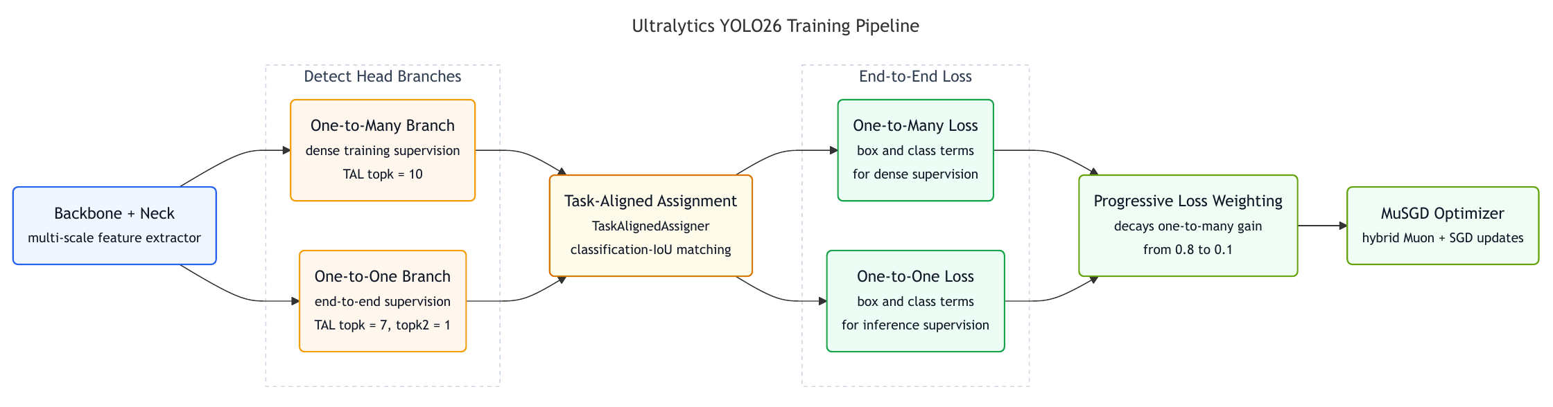
Figure 7. Original YOLO26 Figure 2, by Glenn Jocher and colleagues, arXiv v1, page 6. Cropped from the paper and reused under CC BY 4.0. This is the authors’ high-level training schematic; source-level gradient behavior and current inference defaults require the qualifications below. Figure provenance.11
Two implementation details prevent an overly simple interpretation of that
figure. First, Detect.forward in the inspected release detaches the features
fed to the one-to-one branch during training. Increasing that branch’s loss
weight does not mean it sends an increasing direct gradient into the shared
backbone through that detached path. Second, the report expands candidate
geometry for sides below 8 pixels to 16 pixels; the inspected released assigner
floors sides below 16 to 16. The shared principle is stable, but the exact
candidate rule is version-specific.1711
The released detection recipe is also more than a short COCO fine-tune. The report describes 150 epochs of Objects365-v1 pretraining, followed by size-dependent COCO fine-tuning, with global batch 128. A command that trains for 100 epochs on a small example dataset neither reproduces that recipe nor explains the quality of the released checkpoints.11
Choose the inference path explicitly
The paper calls one-to-one inference the default. The inspected software
release, Ultralytics v8.4.208, uses one-to-many with NMS by default in the
high-level prediction and validation API. Its nms option defaults to None;
setting nms=False selects the one-to-one head where available. The architecture
YAML’s end2end: True declares capability; the runtime setup still selects the
path. The current guide agrees with that source behavior.111725
| Path | High-level API in v8.4.208 | Decoded detection output example | Selection |
|---|---|---|---|
| One-to-many | nms=None or the usual default |
Raw exported detection tensor can be (B, 4+C, A) |
Library runs NMS for prediction/validation; a raw export leaves it to the consumer |
| One-to-one | nms=False |
(B, K, 6): corners, score, class index |
Decode and select top candidates, without IoU-based suppression |
Here B is batch size, C class count, A the number of prediction locations,
and K a selected limit. At 640 × 640, the three-level example has A=8400;
the documented E2E example uses up to 300 predictions per image. Dynamic input,
max_det, task-specific channels and export format can alter the contract.
Segmentation and pose outputs must not be parsed as plain detection tensors.1725
For a frozen software environment, the relevant API distinction is:
from ultralytics import YOLO

model = YOLO("yolo26n.pt")
dense_results = model.predict("image.jpg")             # one-to-many + NMS
e2e_results = model.predict("image.jpg", nms=False)     # one-to-one, NMS-free
This is a documented interface example for ultralytics==8.4.208, not an
experiment run for this article. Loading the model can download weights.
Choose the export path as explicitly as the prediction path: nms=False
selects the NMS-free head; nms=True can embed NMS where supported; default
raw exports can require consumer-side NMS.25
Keep reported accuracy tied to the head
The primary report distinguishes ordinary NMS validation from E2E validation. That distinction is easy to lose when a headline quotes accuracy and NMS-free speed together.
| Scale | COCO AP50–95, one-to-many + NMS | COCO AP50–95, one-to-one E2E | Reported CPU ONNX / T4 TensorRT10 speed, ms |
|---|---|---|---|
| YOLO26n | 40.9 | 40.1 | 38.9 / 1.7 |
| YOLO26s | 48.6 | 47.8 | 87.2 / 2.5 |
| YOLO26m | 53.1 | 52.5 | 220.0 / 4.7 |
| YOLO26l | 55.0 | 54.4 | 286.2 / 6.2 |
| YOLO26x | 57.5 | 56.9 | 525.8 / 11.8 |
Author-reported values, YOLO26 report Table 7, 640-pixel input. The CPU is identified as Intel Xeon at 2.00 GHz; the GPU column is T4 TensorRT10. The release documentation identifies its published speed path as the NMS-free head and the T4 inference format as FP16. These are published inference benchmarks, not full capture-to-result timings. They do not measure NMS latency for the higher-AP branch, and they were not reproduced here.1126
Across these five entries, NMS validation is 0.6–0.8 AP points higher. That is a reported trade-off between two paths from the same family, not evidence that NMS always improves any detector or that one runtime must be faster on every accelerator. The substantial Objects365 pretraining also matters when comparing these models with checkpoints trained only on COCO.
What to watch next
YOLO27 is a preview, with no public weights, configurations or implementation in the inspected official documentation. Its planned design separates compact CNN models from larger query-based models. Those plans are interesting evidence of architectural diversification, but preliminary charts are not measurements of a released artifact we can inspect or deploy.12
The useful 2026 trend is a combination of better representation, richer training and simpler deployment paths. Adding attention and removing a box regression distribution are not contradictory: complexity can be moved to where it buys useful accuracy or training signal, and removed where it adds deployment cost. Whether that trade works is an empirical question for the actual model, input and hardware.
Beyond fixed categories
A standard closed-set detector predicts a fixed category list learned during training. Renaming an output label does not teach it a new visual concept. Open-vocabulary models connect region features to a broader semantic space, allowing categories to be supplied or changed more flexibly.
YOLO-World brings vision-language modeling into a real-time detector. Its RepVL-PAN connects visual features with text information. A useful deployment idea is to prepare vocabulary embeddings ahead of time, so a fixed application vocabulary does not require rerunning a text encoder for every frame.14
YOLOE extends efficient detection and segmentation across three prompt mechanisms: text prompts, visual examples, and a prompt-free mode using a built-in vocabulary. Its named mechanisms—RepRTA, SAVPE and LRPC—address alignment, visual prompting and efficient region/prompt comparison. Prompt-free means an explicit per-request prompt is unnecessary; it does not mean the model has no vocabulary, training assumptions or recognition limits.15
YOLOE-26 applies the YOLOE formulation to the YOLO26 family. The report also describes a stronger text encoder, pseudo-label enrichment and a revised segmentation training procedure. Its open-vocabulary benchmark numbers belong to a different task and protocol from closed-set COCO detection. They should not be inserted into the same AP ranking.11
For a device, ask whether the target concepts change at runtime, whether example images describe them better than names, and whether vocabulary preparation belongs on the device or elsewhere. Open vocabulary expands the interface; it does not guarantee reliable detection of arbitrary objects, attributes or novel defects.
Reading accuracy and speed correctly
IoU, precision, recall and AP
Intersection over union (IoU) measures the overlap between a predicted and reference box:
A true-positive decision requires an appropriate category and a successful match under the evaluation rules. Precision asks what fraction of reported detections are correct; recall asks what fraction of annotated objects were found. Raising a score threshold often removes both false positives and some true positives. Average precision (AP) summarizes the precision/recall relationship as predictions are ranked, rather than describing performance at one arbitrary threshold.
COCO’s headline detection AP averages IoU thresholds from 0.50 to 0.95 in steps of 0.05, across categories under its evaluation rules. AP50 uses only IoU 0.50; it is easier to obtain a high value while boxes are imprecise. Small/medium/large-object AP provides additional slices, and the standard COCO evaluator uses its own detection limits and ignore rules. A model emitting up to 300 boxes does not mean standard COCO AP evaluates 300 final detections per image without a limit.27
Do not equate the original paper’s VOC mAP with contemporary COCO AP50–95. Different datasets, splits, overlap rules and class distributions make those numbers answers to different questions.
A benchmark needs a complete identity
Before comparing two accuracy/speed points, identify:
| Dimension | What must match, or be disclosed |
|---|---|
| Artifact | Author repository, model variant, checkpoint edition and software version |
| Learning | Training data, external pretraining, schedule, augmentation and model selection |
| Accuracy protocol | Dataset/split, metric, input size, head mode, test-time augmentation and detection limits |
| Execution | Exact device, runtime/compiler, precision, input shape, batch size and warm-up |
| Timing boundary | Network only, preprocessing + inference, post-processing, transfers or complete system |
| Operating behavior | Sustained latency, tail latency, queue depth, memory, power and thermal conditions |
A model’s FLOPs do not capture memory traffic, operator support or scheduling. Fewer parameters do not guarantee less latency. An attention kernel can perform well on one GPU and be poorly supported on an accelerator. An NMS-free graph may be easier to compile, but that is not a substitute for checking the actual runtime.
Independent evidence also argues against ranking by version. ODVerse33 compares a v5–v11 cohort across 33 datasets in 11 domains and reports rankings that vary by domain. Its training setup uses a common resolution and schedule, with checkpoint selection choices that still bound the conclusions. The study does not evaluate YOLO26; it supports the narrower lesson that a later name alone is insufficient evidence of application quality.28
From a model to a working system
A useful starting point is a maintained implementation with documented weights and exports, plus a compact baseline you can measure. For new Ultralytics work, YOLO26 is its current released family. For research, the official v10, v12, v13, YOLOX and other author repositories expose different mechanisms worth studying. Choose a question before choosing a model: limited CPU latency, small-object recall, crowded scenes, changing categories or accelerator compatibility can lead to different experiments. Figure 8 places inference inside the complete path to measure.2689104
A fast model is one stage of a responsive device.
Measure the time from a real observation to a useful result, including queues and work outside the neural network.
- 01CaptureExposure, sensor readout, timestamps
- 02PrepareDecode, letterbox, normalize, transfer
- 03InferBackbone, feature fusion, prediction head
- 04SelectDecode, threshold, NMS or top-k; undo padding
- 05UseAssociate tracks, decide, display or act
Capture → prepare → infer → select → use. Record timestamps at the boundaries and distinguish per-frame latency from steady-state throughput. Transfers and queueing can dominate; a model-only millisecond figure is not camera-to-action latency.
Conceptual pipeline, not a device benchmark. Stages can overlap on independent resources; tracking and decisions are separate functions beyond single-frame detection.
Figure 8. Detection inside a complete system. Neural-network inference is one stage; a working device also captures, moves, transforms and uses information. The pipeline is conceptual and has no invented timing measurements. Compare Hardware 101’s timing foundations.
Establish the data and evaluation contract
- Define the output. Classes, box convention, minimum useful object size, allowable misses and false alarms. For tracking, add the identity and temporal requirements separately.
- Build a representative test set. Include lighting, viewpoints, backgrounds, distances and negative scenes from the intended environment. Separate nearby frames, people or capture sessions where leakage would otherwise inflate results.
- Audit labels. Missing objects can make a correct detection appear to be a false positive. Inconsistent class definitions can make training and evaluation disagree.
- Keep a fixed baseline. Record the repository, checkpoint, version, input pipeline and metric. Change one important factor at a time, or disclose that the whole recipe changed.
- Inspect failures. Separate misses, classification errors, duplicate detections and poor localization. Slice by object size, scene and operating condition, not only an aggregate AP value.
A higher-resolution input cannot recover details that the camera never captured. Tiling can make small objects occupy more model pixels, but creates boundary cases and extra work. Removing NMS can eliminate a suppression failure while leaving representation, domain shift or annotation problems unresolved.
Preserve the input/output contract during deployment
Letterboxing preserves aspect ratio by resizing and padding. If the deployed pipeline uses a different resize policy, color channel order, normalization or padding convention than the tested model expects, detections can degrade even though inference succeeds. Box coordinates must be transformed back using the same scale and offsets.
Export the chosen head and task, then compare exported and reference outputs on the same images. Check box order, score interpretation, coordinates, thresholding and class IDs. Test dynamic shapes deliberately; a tensor layout that works for one fixed resolution may fail when a camera changes aspect ratio. Quantization requires its own accuracy and failure review on representative data, rather than an assumption that reduced numerical precision is invisible.
Record the licenses for code, checkpoints and data alongside the artifact identity. The inspected Ultralytics source is labeled AGPL-3.0; a third-party implementation or hosted model can have different terms. The CC BY licenses for the paper figures on this page are separate from model-software and checkpoint licensing.17
Measure the system that will actually run
Measure steady-state throughput and per-frame latency separately. Capture can continue while inference runs, so their reciprocal relationship is not always simple. A queue can preserve every frame while allowing decisions to become increasingly stale. Depending on the application, dropping obsolete frames may produce more useful responses than maximizing processed-frame count.
Report both a typical operating point and tail behavior under the intended load. Include sustained runs, memory use and thermal or power constraints for a device. Check whether an unsupported operator silently falls back to the CPU and whether transfers dominate the time saved by a smaller model. These are engineering questions about the complete implementation, not judgments that can be made from a model’s name.
For deeper foundations, continue with Hardware 101, Edge AI evaluation and profiling, quantization and compression and local/cloud collaboration.
Common misunderstandings
| Misunderstanding | A more useful interpretation |
|---|---|
| “YOLO is one official numbered sequence.” | Identify the author/project and the released artifact; several independent research lines share the name. |
| “One look means no post-processing.” | The original detector used NMS; modern E2E paths can still decode, threshold and select. |
| “Anchor-free means NMS-free.” | Box parameterization and unique-output assignment are different design choices. |
| “All YOLO confidence scores have the same formula.” | Read the head: explicit objectness, class logits and quality-aware targets differ. |
| “The training diagram is the deployed graph.” | Auxiliary paths, reparameterized blocks and removed heads can change the inference structure. |
| “The best AP and best speed describe the same setup.” | Verify head mode, input, pretraining, precision, runtime and timing boundary. |
| “Open vocabulary means anything will be detected.” | The vocabulary interface is broader; reliable recognition still depends on data, concepts and context. |
| “The newest model must be best for my device.” | Compare the real accuracy–latency–memory trade-off on the target workload and hardware. |
Sources and study scope
This is a source-based family study. Original method sections, selected experiments and official artifact records support the explanations. The YOLO26 implementation discussion is pinned to Ultralytics v8.4.208; mutable release status was checked on November 8, 2026. Figure captions distinguish independent teaching diagrams from cropped original artwork.
We did not train or run these models, download their weights, or reproduce their benchmarks. Coverage is selective across the wider ecosystem: the main numbered branches and influential YOLOX/open-vocabulary work receive priority, rather than every specialized YOLO modification. Author-reported measurements are labeled, and the paper/API differences are retained rather than silently resolved in favor of a cleaner story.
References
-
Joseph Redmon, Santosh Divvala, Ross Girshick and Ali Farhadi. You Only Look Once: Unified, Real-Time Object Detection, first submitted June 2015; inspected arXiv v5, May 2016. Sections 1–2.4 and original architecture/training/inference definitions. ↩ ↩2 ↩3 ↩4 ↩5 ↩6 ↩7
-
Alexey Bochkovskiy, Chien-Yao Wang and Hong-Yuan Mark Liao. YOLOv4: Optimal Speed and Accuracy of Object Detection, April 2020. Architecture and training recipe; author Darknet repository. ↩ ↩2 ↩3
-
Ultralytics. YOLOv5 repository, v7.0 README. Tagged model/workflow evidence for the original project, rather than current v5u outputs. ↩ ↩2
-
Zheng Ge, Songtao Liu, Feng Wang, Zeming Li and Jian Sun. YOLOX: Exceeding YOLO Series in 2021. Section 2; official Megvii implementation. ↩ ↩2 ↩3 ↩4 ↩5 ↩6 ↩7 ↩8
-
Chuyi Li and colleagues. YOLOv6: A Single-Stage Object Detection Framework for Industrial Applications, September 2022; YOLOv6 v3.0: A Full-Scale Reloading, January 2023, Sections 1–2. Official Meituan repository. ↩ ↩2
-
Chien-Yao Wang, Alexey Bochkovskiy and Hong-Yuan Mark Liao. YOLOv7: Trainable bag-of-freebies sets new state-of-the-art for real-time object detectors, July 2022. Sections 3–4; author repository. ↩ ↩2
-
Chien-Yao Wang, I-Hau Yeh and Hong-Yuan Mark Liao. YOLOv9: Learning What You Want to Learn Using Programmable Gradient Information, February 2024. Sections 4.1–4.2; author repository. ↩ ↩2
-
Ao Wang, Hui Chen, Lihao Liu, Kai Chen, Zijia Lin, Jungong Han and Guiguang Ding. YOLOv10: Real-Time End-to-End Object Detection, May 2024. Sections 3.1–3.2 and Figure 2; official THU-MIG implementation. ↩ ↩2 ↩3 ↩4 ↩5 ↩6 ↩7 ↩8 ↩9
-
Yunjie Tian, Qixiang Ye and David Doermann. YOLOv12: Attention-Centric Real-Time Object Detectors, February 2025. Sections 3.2–3.3; official author repository. ↩ ↩2 ↩3 ↩4
-
Mengqi Lei and colleagues. YOLOv13: Real-Time Object Detection with Hypergraph-Enhanced Adaptive Visual Perception, first submitted June 2025; inspected September 2025 revision. Section III A–B; official iMoonLab repository. ↩ ↩2 ↩3 ↩4
-
Glenn Jocher, Jing Qiu, Mengyu Liu, Shuai Lyu, Fatih Cagatay Akyon and Muhammet Esat Kalfaoglu. Ultralytics YOLO26: Unified Real-Time End-to-End Vision Models, June 2, 2026. Sections 3.1–3.3, 3.6, 4.1–4.4 and Table 7; selected supplementary training details. Figure 2 reused under CC BY 4.0. ↩ ↩2 ↩3 ↩4 ↩5 ↩6 ↩7 ↩8 ↩9 ↩10 ↩11
-
Ultralytics. YOLO27 preview documentation at v8.4.208, checked November 8, 2026. No public weights, configurations or implementation; architecture and benchmarks are preliminary. ↩ ↩2 ↩3
-
YOLOv14 arXiv record, checked November 8, 2026. Authors withdrew version 4 on August 20, 2026; its results are not treated as an active successor benchmark here. ↩ ↩2 ↩3
-
Tianheng Cheng and colleagues. YOLO-World: Real-Time Open-Vocabulary Object Detection, 2024. Primary abstract and official author repository for the bounded overview of RepVL-PAN and vocabulary preparation. ↩ ↩2
-
Ao Wang, Lihao Liu, Hui Chen, Zijia Lin, Jungong Han and Guiguang Ding. YOLOE: Real-Time Seeing Anything, March 2025. Primary abstract and official author repository for text, visual and prompt-free modes. ↩ ↩2
-
Ultralytics. YOLO26 public launch announcement, January 14, 2026. Distinguish the public launch from its 2025 introduction and June 2026 paper submission. ↩ ↩2
-
Ultralytics. Released source v8.4.208: YOLO26 YAML, Detect head, E2ELoss, assigner, predictor, validator, NMS utilities, defaults and LICENSE. Read-only source inspection; no model execution. ↩ ↩2 ↩3 ↩4 ↩5 ↩6 ↩7 ↩8 ↩9 ↩10 ↩11 ↩12
-
Joseph Redmon and Ali Farhadi. YOLOv3: An Incremental Improvement, April 2018. Sections 2.1–2.5 and scale-specific prediction contracts. ↩ ↩2 ↩3 ↩4
-
Joseph Redmon and Ali Farhadi. YOLO9000: Better, Faster, Stronger, December 2016. Sections 2–4: priors, multi-scale training and hierarchical joint supervision. ↩ ↩2
-
Nicolas Carion and colleagues. End-to-End Object Detection with Transformers, 2020. Abstract: set prediction, bipartite matching and object queries. ↩ ↩2
-
Ultralytics. YOLOv5 / YOLOv5u documentation, checked November 8, 2026. Original release month, updated head and checkpoint compatibility distinction. ↩
-
Ultralytics. YOLOv8 documentation at v8.4.208. January 10, 2023 release and split anchor-free head. ↩
-
Ultralytics. YOLO11 documentation at v8.4.208. September 27, 2024 software release; model YAML. ↩
-
Yian Zhao and colleagues. DETRs Beat YOLOs on Real-time Object Detection, first submitted 2023. Abstract: efficient hybrid encoder and query-based alternative; no cross-paper speed ranking inferred here. ↩
-
Ultralytics. End-to-end detection guide at v8.4.208.
nms=None/True/False, head choice, output formats and export behavior. ↩ ↩2 ↩3 -
Ultralytics. YOLO26 documentation at v8.4.208. Model availability, published benchmark qualifiers, task family and head-mode description. ↩ ↩2
-
Piotr Dollár and Tsung-Yi Lin / COCO contributors. Official COCO evaluator,
Params.setDetParams, matching andsummarize. IoU thresholds, area ranges, recall thresholds and maximum-detection conventions. ↩ -
Tianyou Jiang and Yang Zhong. ODVerse33: Is the New YOLO Version Always Better? A Multi Domain benchmark from YOLO v5 to v11, February 2025. Sections 3.2, 4 and conclusions; findings are limited to the tested cohort and protocol. ↩