The first Edge AI question is not “How large a model can this device load?” It is “Can this device complete the useful task, reliably, within its budgets?” A compact checkpoint is only part of that answer. Model state, temporary tensors, input processing and the runtime also need space and time. Mobile deployment guidance explicitly separates storage, memory, performance and execution-provider choices.1
For a hardware introduction and current device platforms, read On device computing.
Use this page to form a budget before optimizing. Its numerical examples are hypothetical calculations, not measurements of a particular model or device.
Start from the workload
A short voice command, a document question and continuous camera perception are different workloads. State the input size, expected output, arrival pattern, quality threshold and deadline. Then ask what must remain available while the task runs.
Five budgets, not one model-size limit
5 budgets| Budget | Useful question | What to carry into a test |
|---|---|---|
| Capability | Does the output solve the task? | Acceptance criteria, important failure slices and abstention behavior |
| Capacity | What must coexist in memory? | Resident weights, cache, live tensors, workspace and application state |
| Movement and compute | Where is time actually spent? | Bytes transferred, kernel work, copies and processor transitions |
| Responsiveness | When does the user get a useful result? | Cold start, first useful output, completion and cancellation |
| Sustained operation | Does repeated use remain acceptable? | Temperature, battery state, energy and competing application load |
No matching budgets. Try another term or reset the search.
Scroll to compare. Focus view gives the table more room.
This is a proposed design checklist, not a universal benchmark standard. MCUNet shows why device regime matters: its microcontroller study jointly designed the network and inference engine for severe memory constraints.2 A phone or laptop has different resources and system behavior. Do not transfer a result between these regimes without testing the relevant workload.
Stored weights are the first estimate
For stored parameter values represented at bits each, the ideal weight payload in bytes is:
This is representation arithmetic. A hypothetical dense 3 billion parameter model at four bits per value has a 1.5 GB weight payload, about 1.40 GiB. GB here means bytes; GiB means bytes. Packing, scales, zero points, unquantized tensors and file metadata can increase the actual size.
The number of parameters stored matters here. A sparse model’s active parameter count describes selected computation, not permission to omit the other expert weights from its storage budget. See efficient architectures.
Context is another growing allocation
An ordinary autoregressive Transformer caches attention keys and values so it can reuse past states. Grouped query attention (GQA) shares those states among query heads, reducing their size relative to separate KV heads for every query head.3
For a uniform full-context decoder cache, the ideal payload in bytes is:
| Symbol | Meaning |
|---|---|
| Number of layers storing this cache | |
| Number of sequences cached concurrently | |
| Stored token positions per sequence, including generated tokens | |
| Stored key and value heads, not the query-head count | |
| Key and value head width, assumed equal | |
| Bits per stored cache value |
The factor two is for keys and values. This is a local shape derivation from the ordinary attention contract, not an implementation’s allocation report.3 Sliding windows, different layer types, compressed latent attention and recurrent state require their own accounting. Allocators may also reserve more positions than are currently occupied.
Work through a hypothetical budget
Assume one sequence, 28 cached layers, eight KV heads, head width 128 and 16 bit cache values. These are illustrative inputs, not a named checkpoint.
Figure 1 adds the fixed weight payload to each cache case.
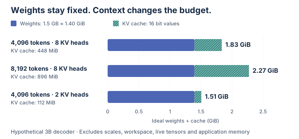
Figure 1. Context changes ideal weight-plus-cache payload. Calculated here from the hypothetical budget.3
The three cache values are 448 MiB, 896 MiB and 112 MiB, calculated from Equation (2). With the 1.5 GB weight payload, the baseline already needs about 1.83 GiB for weights and cache alone. That does not prove it fits a 3 GiB application budget: the next step is to account for everything else that is live at the same time. Nor does the smaller cache prove equal task quality or supported fast kernels.
Peak memory follows lifetimes
Do not add a model file to every tensor ever created. Add the allocations that coexist, then take the largest total over time:
Equation (3) is a bookkeeping model. Define categories without double counting; include duplicated buffers, reservations and application allocations in the measured budget. Here the cache term means allocated storage, including reserved capacity, not only Equation 2’s occupied payload. Device and process accounting can expose different views.
ExecuTorch’s memory planner tracks tensor sizes and lifetimes to assign buffers. With bounded dynamic shapes, planning may use upper-bound sizes rather than the current input’s occupied size.4 Figure 2 follows the allocations through a request.
- LoadWeights, mappings and runtime initialization
- PrefillPrompt states, temporary tensors and growing KV cache
- DecodeResident weights, cache and per-step workspace
- Release or reuseFree task state or retain a bounded cache
A vision or audio encoder may add a separate peak. Profile whether its buffers coexist with decoder state.
- Tensor lifetimesWhen each intermediate is needed
- Buffer assignmentReuse storage for tensors whose lifetimes do not overlap
- Actual peakCheck reservations, backend workspace and application load
Figure 2. Peak memory depends on overlapping allocations. Independent lifecycle synthesis informed by memory planning and decoder-cache methods.43
Storage outside DRAM can extend capacity, but it creates an I/O problem. Apple’s LLM in a Flash summary describes loading selected parameters from flash and organizing reads around reuse and contiguous bundles. It does not establish that arbitrary offloading is fast.5
Compute and bandwidth are different bottlenecks
The Roofline view compares arithmetic with data movement. For a fixed workload, let be operation count, bytes moved at the memory level being studied, attainable operation throughput and attainable bandwidth. An optimistic lower bound is:6
This local adaptation assumes ideal overlap and ignores additional overhead. Use matching operation types and precision: advertised INT8 TOPS is not an FP16 FLOP/s budget. Arithmetic intensity is operation count per byte; the relevant memory level and attainable limits matter.6
Figure 3 shows the original visual argument. On the left, low operational intensity reaches the sloped memory ceiling before the flat compute ceiling. On the right, the authors compare Opteron X2 and X4: more arithmetic capacity does not give the same gain to workloads near the memory slope. These are historical CPU examples, not phone or NPU results.7
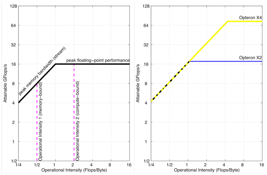
Figure 3. Historical Roofline examples. Cropped from Williams, Waterman and Patterson, Figure 1 (2008), with both panels retained.78
For one sequence using ordinary one-token-per-step decoding, assume all 1.5 GB of packed weights must be read once from memory per step at an effective 30 GB/s. Weight traffic alone takes at least 50 ms, giving a ceiling of 20 tokens/s under those assumptions. Actual step time can be higher because of cache traffic, compute, dequantization and synchronization; some of that work may overlap. This is not a device prediction. Batching, multi-token verification or a different access pattern changes the premise.
GQA’s motivation includes memory-bandwidth costs during incremental decoding.3 Processing many prompt positions together and generating one position at a time are different workloads. Use the inference chapter to separate them before choosing an optimization.
Turn the budget into a measurement contract
Suppose the product asks for a short answer to a local document question. A useful test record would specify the device and software versions, document input, prompt and output limits, quality target, cold and warm conditions, peak memory, first useful output, completion time and repeated use conditions. This is a proposed experiment, not one we performed.
MLPerf Mobile pairs defined workloads with quality targets and scenario metrics. Its structure is a useful reminder that “fast” needs a task and quality contract, although a benchmark is not the complete product experience.9
Three traps are worth checking explicitly:
- The file fits, the workload does not. Test the maximum supported context and input shape, not only a short demonstration.
- The accelerator exists, the graph does not stay on it. Unsupported operators can split execution across providers; measure the resulting path rather than assuming acceleration.1
- The first run is good, sustained use is unknown. Keep isolated inference results separate from the repeated workload the product needs.
The next move follows the failing budget. Use compression for representations, runtimes for backend support, and evaluation for actual measurements. If the useful task still does not fit, reconsider its scope or use a bounded hybrid system.
References
-
ONNX Runtime, Deploy on mobile, storage, memory, execution providers and partitioning. Inspected October 12, 2026. ↩ ↩2
-
Ji Lin et al., MCUNet, official summary of the TinyNAS and TinyEngine co-design, NeurIPS 2020. ↩
-
Joshua Ainslie et al., GQA: Training Generalized Multi-Query Transformer Models from Multi-Head Checkpoints, Introduction and Section 2.2; v3, December 23, 2023. The paper’s experiments use T5 variants, not a universal edge-device benchmark. ↩ ↩2 ↩3 ↩4 ↩5
-
PyTorch, ExecuTorch memory planning, tensor lifetimes, dynamic-shape bounds and buffer planning; documentation identified as version 1.5 when inspected October 12, 2026. ↩ ↩2
-
Keivan Alizadeh et al., LLM in a Flash: Efficient Large Language Model Inference with Limited Memory, Apple’s official research summary, ACL 2024. The summary, not the full experimental paper, is the inspected source here. ↩
-
NERSC, Roofline Performance Model, performance envelope, attainable hardware limits and arithmetic intensity. Inspected October 12, 2026. Equation 4 is a local time-bound adaptation, not a reported device result. ↩ ↩2
-
Samuel Williams, Andrew Waterman and David Patterson. Roofline: An Insightful Visual Performance Model for Floating-Point Programs and Multicore Architectures, UCB/EECS-2008-134, October 17, 2008. Section 3 and Figure 1, PDF page 4 (printed page 2). The caption is omitted from the image crop; plots, axes and labels are unchanged. ↩ ↩2
-
Figure sources and reuse assessment. The report retains copyright 2008 by its authors; the selected figure is included for specific criticism and review, not relicensed under MIT. ↩
-
MLCommons, MLPerf Inference: Mobile, scenario metrics and quality targets. Inspected October 12, 2026. ↩